Accuracy of the FPGA Math & Analysis VIs
Overview
- Quantization errors due to limited precision fixed-point arithmetic
- Underflow errors introduced in signal paths with large dynamic range
- Overflow errors if the input signal violates design assumptions
- Disabling measurement features such as windowing and interpolation in order to conserve resources on the FPGA
Conversely, some parts of the FPGA implementation can actually be more accurate than the equivalent floating-point implementation because internal 64-bit integer data paths allow us to retain more significant bits than the 53 bits provided by the double precision floating-point data type.
Contents
DC and RMS Measurements
The DC and RMS Measurements FPGA VI offers several options for calculating the DC and RMS values of a 16-, 24-, or 32-bit input with or without the Apply Hanning window option enabled. The accuracy of the measurement result depends on the input and windowing option you select. Refer to the tables and graphs below for more details on the specifications under the different conditions.
The DC and RMS Measurements VI takes an integer input signal and returns integer result values. While the accuracy specifications cannot account for the initial quantization of the input signal before it is passed to the measurement VI, the specifications do account for the re-quantization error (+/- 0.5 LSB) caused by the rounding of the result to an integer value. In other words, the specifications describe the differences between the returned results and the floating-point calculations based on the same integer input signal data.
Error Sources
Since windowing involves extra computation, the use of a window will add slightly to the numerical error due to quantization effects. The fixed-point implementation of the Hanning window uses sufficient precision such that the computation is not a significant source of error in the overall measurement algorithm.
For 32-bit inputs, the RMS, mean square, and square sum measurements do not retain the full 78-bit internal precision required to produce an exact accumulation result for full-scale input signals. In this situation, the design must either allow the possibility of overflow (where large input signals cause the result to wrap or saturate) or underflow (where precision is lost due to downscaling; small input signals are scaled down to zero and have no effect on the result). The DC and RMS measurement implementation in this case guarantees that no overflow will occur, but it allows underflow when scaling the signal down to fit in a 64-bit integer. To minimize the effects of this, use the smallest bitwidth implementation appropriate for your signal. For example, if you have a 32-bit integer data path but know that the signal will never have a magnitude larger than 32767, you should convert the signal to an I16 and use the 16-bit RMS measurements.
Note that the DC and RMS Measurements VI optimizes calculations such that the errors are small compared to gain and offset errors originating from typical acquisition hardware. Therefore, when evaluating the different error sources in the measurement chain, you can often discard the following calculation errors.
Error Specifications
Configuration
| Error
(Percent of Result +/- LSBs) | Reference Graph
|
| 16 bit – Windowing disabled | +/- 1.0
| Graph 1
|
| 16 bit – Windowing enabled | +/- 1.5
| Graph 1
|
| 24 bit – Windowing disabled | +/- 0.002% +/- 1.5
| Graph 2
|
| 24 bit – Windowing enabled | +/- 0.003% +/- 3.0
| Graph 2
|
| 32 bit – Windowing disabled | +/- 0.002% +/- 1.5
| Graph 3
|
| 32 bit – Windowing enabled | +/- 0.003% +/- 3.0
| Graph 3
|
Table 1: DC Calculation Error Relative to Floating-Point Result
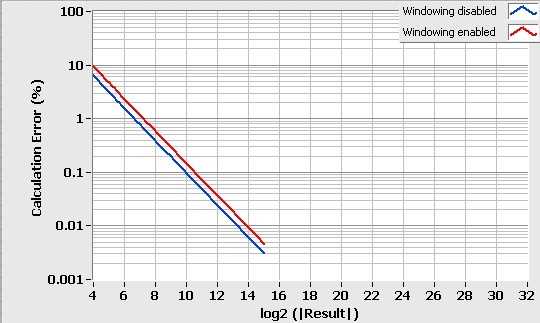
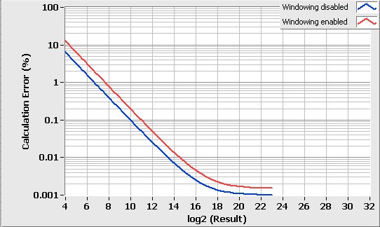
Graph 1: DC Calculation Error for 16-bit Input
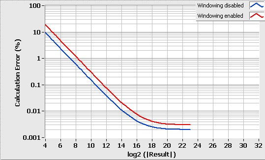
Graph 2: DC Calculation Error for 24-bit Input
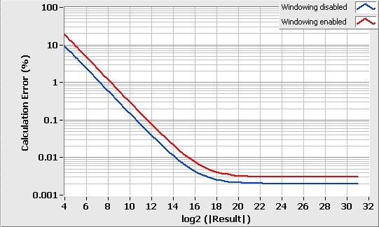
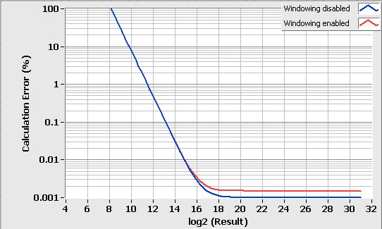
Graph 3: DC Calculation Error for 32-bit Input
Configuration
| Error
(Percent of Result +/- LSBs) | Reference Graph
|
| 16 bit – Windowing disabled | +/- 1.0
| Graph 4
|
| 16 bit – Windowing enabled | +/- 1.0
| Graph 4
|
| 24 bit – Windowing disabled | +/- 0.0010% +/- 1.0
| Graph 5
|
| 24 bit – Windowing enabled | +/- 0.0015% +/- 2.0
| Graph 5
|
| 32 bit – Windowing disabled | Refer to Graph
| Graph 6
|
| 32 bit – Windowing enabled | Refer to Graph
| Graph 6
|
Table 2: RMS Calculation Error Relative to Floating-Point Result
Graph 4: RMS Calculation Error for 16-bit Input (with and without windowing)
Graph 5: RMS Calculation Error for 24-bit Input
Graph 6: RMS Calculation Error for 32-bit Input
Analog Period Measurement
Interpolation
A standard threshold crossing detection scheme for period measurements provides linear interpolation at the crossing in order to estimate the precise instant of the crossing with sub-sample accuracy. Implemented in the FPGA, however, the interpolation operation requires a division operation that takes one clock cycle per bit of accuracy to execute. In cases where speed is critical, accuracy is not critical, or interpolation provides no benefit, you may disable the interpolation feature to save FPGA resources.
The Analog Period Measurement VI computes the interpolated sample fraction to 8-bit accuracy. In most cases, this introduces significantly less error than the assumption that the signal is exactly linear between the two samples that cross the threshold. The format of the output samples (x 2^16) contains 16 fractional bits, however, to allow for the improved accuracy obtainable by averaging over multiple signal periods.
Averaging
This feature allows you to trade off measurement time for accuracy by measuring the time duration of multiple periods of the input signal and returning an average period over the interval. The number of periods is restricted to be a power of 2 in order to provide an efficient hardware implementation. This setting assumes that the input signal frequency is stable during the measured interval. If this condition is met, the error is inversely proportional to the number of periods measured.
Butterworth Filter
The Butterworth Filter FPGA VI includes the following specifications:
- Supported types - Lowpass and highpass filters
- Supported orders - First, second, and fourth order filters
- Supported input resolutions - 16, 24, and 32 bit
- Lowpass filter gain at DC - 1.000 (0.00 dB)
- Highpass filter gain at Nyquist frequency1 - 1.000 (0.00 dB)
- Filter gain at Cutoff freq.(Hz) - 0.707 (-3.01 dB)
- Normalized cutoff frequency range2 - 10-6 to 0.49
1 The Nyquist frequency is defined as Expected sample rate/2.
2 The normalized cutoff frequency is defined as the ratio Cutoff frequency/Expected sample rate and is unit-less.