NI does not actively maintain this document.
This content provides support for older products and technology, so you may notice outdated links or obsolete information about operating systems or other relevant products.

Read this whitepaper to learn about the challenges facing today's multicore programmers. Specifically, this document discusses a breadth of multicore programming patterns that may be applied to a software architecture.
Several books thoroughly examine programming patterns, so this document introduces at a high-level the following concepts and how they may be applied in LabVIEW:
1. Task Parallelism
2. Data parallelism
3. Pipelining
4. Structured grid
From a software architecture perspective, try to incorporate a parallel pattern that best suits the application problem. Before you choose the appropriate pattern, consider both application characteristics and hardware architecture.
In addition, various LabVIEW structures will be highlighted in the context of the above-listed patterns (regular while loops, feedback nodes, shift registers, timed loops, and parallel for loops).
The LabVIEW 2014 Real-Time Module includes support for CPUs with up to 12 cores on Phar Lap ETS targets. Previously, the module supported only eight CPU cores even if the target had more available.
Task parallelism is the simplest form of parallel programming, where the application is divided into unique tasks that are independent of one another and can execute on separate processors. Consider a program with two loops (loop A and loop b) where loop A performs a signal processing routine and loop b performs updates to the user interface. This represents task parallelism, whereby a multithreaded application can run the two loops in separate threads to utilize multiple CPUs.
In LabVIEW, task parallelism is achieved by having parallel portions of code on your block diagram. The advantage of LabVIEW is that you can "see" the parallelism in your code and easily separate unique tasks to achieve this form of parallelism. In addition, LabVIEW will automatically multithread your application so you don't have to worry about thread management or synchronization between threads.
You can apply data parallelism to large data sets by splitting up a large array or matrix into subsets, performing the operation, and combining the result.
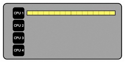
First, consider the sequential implementation, where a single CPU attempts to process the entire data set.
Figure - Single CPU Processing
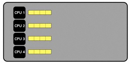
Instead, consider the next example of the same data set split into four parts. You can spread this data set across the available cores to achieve a significant increase in speed.
Figure - Multiple CPU Processing
In real-time high-performance computing (HPC) applications such as control systems, a common and efficient strategy is the parallel execution of matrix-vector multiplications of considerable size. Typically, the matrix is fixed, and you can decompose the matrix in advance. Measurements gathered by sensors provide the vector on a per-loop basis. For example, you can use the result of the matrix-vector to control actuators.
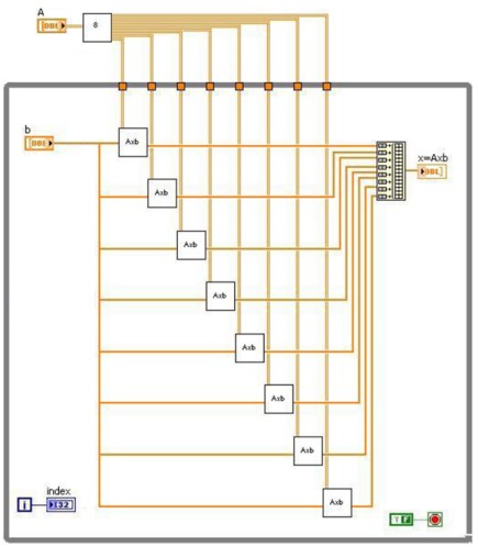
The following block diagram shows a matrix-vector multiplication distributed to eight cores.
Figure - Matrix vector multiplication in LabVIEW
The block diagram executes from left to right and performs the following steps:
1. Splits matrix A before it enters the while loop
2. Multiplies each portion of matrix A by the vector b
3. Combines the resulting vectors to create the final result x=Axb
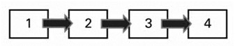
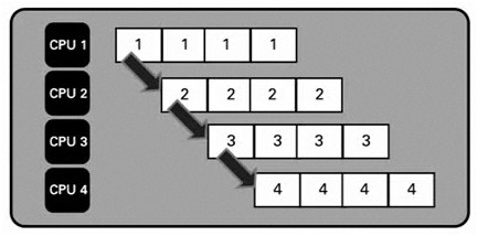
Pipelining is similar to an assembly line. Consider this approach in streaming applications and any time you must modify a CPU-intensive algorithm in sequence, where each step takes considerable time.
Figure - Sequential Stages of an Algorithm
Like an assembly line, each stage focuses on one unit of work. Each result passes to the next stage until the final stage.
To apply a pipelining strategy to an application that will run on a multicore CPU, break the algorithm into steps that have roughly the same unit of work and run each step on a separate core. The algorithm can repeat on multiple sets of data or on data that streams continuously.
Figure - Pipelined Approach
The key is to break up the algorithm into steps that take equal time because each iteration takes as long as the longest individual step in the overall process. For example, if step 2 takes one minute to complete but steps 1, 3, and 4 each take 10 seconds, the entire iteration takes one minute to complete.
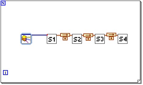
The LabVIEW block diagram in Figure 4 shows an example of the pipelining approach. A for loop appears with a black border and contains stages S1, S2, S3, and S4, which represent the functions in the algorithm that must run in sequence. Because LabVIEW is a structured dataflow language, the output of each function passes along the wire to the input of the next.
Figure - Pipelined Approach in LabVIEW
Note that a Feedback Node appears as an arrow above a small dot. Feedback Nodes denote a separation of the functions into separate pipeline stages. A nonpipelined version of the same code looks similar but without the Feedback Nodes. Examples that commonly use this technique include streaming applications where fast Fourier transforms (FFTs) require manipulation one step at a time.
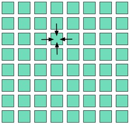
Many computations that involve physical models use a structured grid pattern. In this pattern, you calculate a 2D, or ND, grid every iteration, and each updated grid value is a function of its neighbors, as shown in Figure 8.
Figure - Structured Grid Approach
With a parallel version of a structured grid, you split the grid into subgrids and compute each subgrid independently. Communication between workers is only the width of the neighborhood. Parallel efficiency is a function of the area-to-perimeter ratio.
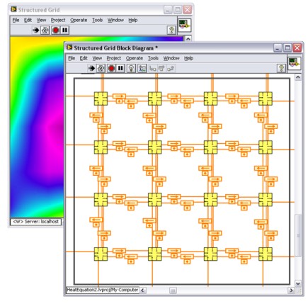
For example, the block diagram in the following figure can solve the heat equation, where the boundary conditions constantly change.
Figure - Structured Grid Approach in LabVIEW
The 16 visible icons represent tasks that can solve the Laplace equation of a certain grid size, where the Laplace equation is a way to solve the heat equation. The 16 tasks map to 16 cores. Once per iteration of the loop, those cores exchange boundary conditions, and the process builds up a global solution. The Feedback Nodes, which appear as arrows above small dots, represent data exchange between elements. You can also map such a block diagram to a one-, two-, four-, or eight-core computer. As computers with greater numbers of cores become available, you can use a similar strategy.
While loops are a fundamental structure that can be used with a variety of programming patterns (task parallelism, data parallelism, pipelining, or structured grid). Depending on the pattern, a regular while loop will suffice, or in other situations a specialized type of while loop (such as the timed loop) may be appropriate.
For the pipelining approach outlined above, either shift registers or feedback nodes should be used (their behavior is the same in this scenario).
The parallel for loop allows you to programmatically set the number of parallel “workers” that execute your code to achieve implicit parallelism (i.e. the code abstracts the complexity and maps different workers to different cores). Create a worker for each processor core to maximize your parallel execution.
The Parallel For loop is a valid approach for intensive operation that needs to execute over and over in loop, without having dependencies from one iteration to the next. However, if there are dependencies, the Parallel For loop should not be used because the dependencies imply that the algorithm should be executed sequentially. In that case, you another technique such as pipelining to achieve parallelism.
The timed loop acts as a while loop but has special characteristics that can help you optimize performance based on the multicore hardware configuration. For example, unlike a regular while loop which may utilize multithreads, any code enclosed within the timed loop executes in a single thread. This may seem counter intuitive, and one might wonder why single thread execution would be desirable on a multicore system. In particular, it's a useful characteristic on real-time systems and where optimizing for cache is important. In addition to executing in a single thread, the loop can set processor affinity, which is a mechanism to assign that thread to a particular CPU (and hence help optimize for cache).
It's important to note that parallel patterns that work well within a regular while loop (such as data parallelism and pipelining), will not work with a timed loop, because no parallelism can be achievable in a single thread. Instead, the techniques can be implemented using multiple timed loops, for example, with pipelining one timed loop can represent a unique stage in the pipeline, with data transfer between loops via FIFOs.
Queues are important for synchronizing data between multiple loops. For example, they can be used to implement a producer/consumer architecture. The producer/consumer architecture was not mentioned in this document specifically, due to the fact that it's not unique to parallel programming and is more of a general purpose programming architecture. Nonetheless it works quite well on multicore CPUs to minimize CPU usage, and the combination of loops and queues make it all possible.
Note that queues are not a deterministic mechanism to share data between loops, if real-time is required use RT FIFOs instead.
Specific to LabVIEW Real-Time, CPUs can be "reserved" for certain thread pools using CPU Pool VIs. This is another mechanism to optimize for cache.
For example, imagine an application will be executed on a quad-core system, whereby the application is intended to operate on data as quickly as possible over and over again. This type of operation is ideal to run in cache, assuming the dataset will actually fit in the CPU cache. In fact, running the operation in cache may be more effective than attempting to parallelize the code and utilize all four CPUs. So, instead of allowing the OS to schedule parallel tasks across all four CPUs (0-3), the developer may choose to reserve only two CPUs for the OS scheduler, such as CPU 0 and 2. (Perhaps the quad-core in question has a large shared cache between CPU 0 and 1, and another large shared cache between CPU 2-3) By reserving CPUs, the developer can help ensure the data stays in cache, and also ensure that the two large shared caches are at full disposal to be used by the operation.
The CPU Information VIs provide information specific to the system the LabVIEW application is running on. This information is very useful if the application may be deployed on a myriad of different machines (such as dual-cores, quad-cores, or even octal cores.
By using the CPU Information VIs, the application can read parameters such as "# of logical processors" and based on the result on a given machine, use that result to feed into a parallel For loop.
For example, if the application is running on a dual-core machine, the # of logical processors = 2, and therefore the optimal number setting for the parallel For loop would also be two. This allows for code to more easily adapt to the underlying hardware.
Tracing is a very useful way to debug multicore applications, and can be performed on both the desktop or a real-time system. Refer to the product documentation for the Desktop Execution Trace Toolkit and the Real-Time Trace Viewer. In LabVIEW 2013 and prior releases of the LabVIEW Real-Time Module, the Real-Time Trace Viewer is packaged as a separate toolkit (Real-Time Execution Trace Toolkit).
To conclude, savvy programmers should consider a programming pattern that will map well to the given application. Patterns discussed in this paper included task parallelism, data parallelism, pipelining, and structured grid.
In order to fully utilize the patterns described in this paper, LabVIEW developers should incorporate different structures, VIs, and debugging tools to ensure optimal performance.