Spline Interpolation
- 업데이트 날짜:2026-05-26
- 2분 (읽기 시간)
Spline interpolation provides a more accurate representation of functions compared to polynomial interpolation by using more data points.
Spline interpolation avoids the disadvantages of polynomial interpolation because functions require more data points and the line interpolant is similar to the original function.
Cubic spline interpolation is a common type of spline interpolation that uses a third-order polynomial for each interval between two adjacent points. Third-order polynomials must meet the following conditions:
- The first and second derivatives at interior points are continuous.
- The polynomials pass through all data points.
- For one-dimensional interpolation, the second derivatives for the beginning and end points are zero. For spline interpolant, the initial boundary and final boundary inputs specify the first derivatives at the beginning and end points. For spline interpolation, a line with the first derivatives behaves the same as the spline interpolant. For spline interpolation, a line with a natural spline behaves the same as one-dimensional interpolation.
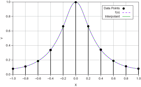
For example, the equation
with natural cubic spline interpolation is shown in the following figure.

When you have more data points of fx, the interpolant of the cubic spline interpolation is similar to fx, as shown in the following figure.
Related information