TSA Independent Component Analysis (Array) VI
- Updated2024-07-30
- 6 minute(s) read
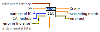
Performs independent component analysis (ICA) on a multivariate (vector) time series. Wire data to the Xt input to determine the polymorphic instance to use or manually select the instance.
Inputs/Outputs
 advanced settings
—
advanced settings
—
advanced settings specifies the iteration settings for independent component analysis. This option is available only when ICA method is Fast ICA.
 Xt
—
Xt
—
Xt specifies the multivariate (vector) time series. Each column of the 2D array represents a vector at certain time.  number of IC
—
number of IC
—
number of IC specifies the number of independent components to estimate. The default is -1, which specifies that this VI computes all the possible independent components.  ICA method
—
ICA method
—
ICA method specifies the method to use in computing the independent components of the multivariate (vector) time series.  error in (no error)
—
error in (no error)
—
error in describes error conditions that occur before this node runs. This input provides standard error in functionality.  instrumental filter
—
instrumental filter
—
instrumental filter specifies the instrumental finite impulse response (FIR) filter coefficients when performing independent component analysis. This option is available only when ICA method is Matrix Pencil ICA. This VI uses the default filter if you do not specify a value for this parameter.  Xt out
—
Xt out
—
Xt out returns the estimated independent components. Each column of the 2D array represents a series of the estimated independent components.
separating matrix
—
separating matrix returns the estimated matrix this VI uses to separate the independent components from the multivariate (vector) time series.  error out
—
error out
—
error out contains error information. This output provides standard error out functionality. |
 convergence tolerance
—
convergence tolerance
—
TSA Independent Component Analysis Details
Independent component analysis (ICA) generates a new set of statistically independent multivariate (vector) time series from the original multivariate time series that are statistically dependent on each other.
You can use the following two methods to perform ICA: Fast ICA and Matrix Pencil ICA. The Fast ICA method adjusts the separating matrix to maximize the negentropy. The Matrix Pencil ICA method calculates the general eigenvector of a matrix pencil formed by two matricesthe auto-correlation matrix of the measurements and the auto-correlation matrix of the measurements filtered by a specified finite impulse response (FIR) filter. The Matrix Pencil ICA method sorts the independent components before returning them. Therefore, the order of the resulting independent components and the signal shape of Xt out when you plot Xt out on a waveform graph are not subject to changes in the number of independent components number of IC. Moreover, the signal shape of Xt out changes with respect to scale only.
This VI implements the Fast ICA method according to the following steps:
1. Calculates negentropy
Negentropy measures nongaussianity of a time series. This VI calculates negentropy for each independent component according to the following equation:
J(yi) = [E{G(yi)} - E(v)]², i = 1,…, n
where n is number of IC, yi is independent components, v is a Gaussian variable of zero mean and unit variance, and G is any non-quadratic function you specify in method.
When method is Square:

When method is Cube:

When method is Tanh:

When method is Gaussian:

2. Maximizes negentropy
Each independent component yi can be represented by input time series Xt multiplied by coefficients in the separating matrix. You can obtain the maximum value for negentropy by adjusting the coefficients in separating matrix with the Newton optimization method.
This VI implements the Matrix Pencil ICA method according to the following steps:
1. Filters the time series by a selected FIR filter and forms the matrix pencil
This VI applies the specified instrumental filter to each channel of the time series and then calculates the autocorrelation of the original time series and the filtered ones. The filter must keep some significant frequency band of the time series but cannot be an all-pass filter. You can calculate the autocorrelation with different delays and then average them to mitigate the effect of noise. The two averaged correlation matrices form the matrix pencil. The following equations describes these steps:
Xt' = filter(Xt)


where bk is the weight, and k is the delay. bk and k are fixed values.
2. Calculates the general eigenvector of the matrix pencil
RXXE = RX'X'ED
where E is the matrix of eigenvectors and D is a diagonal matrix. When the elements of D are distinct, ET is the separating matrix.
Examples
Refer to the following VIs for examples of using the TSA Independent Component Analysis VI:
- Independent Component Analysis VI: labview\examples\Time Series Analysis\TSAGettingStarted
- Magneto Encephalogram (MEG) Signal Analysis VI: labview\examples\Time Series Analysis\TSAApplications