ODE Runge Kutta 4th Order VI
- Updated2025-07-30
- 4 minute(s) read
Solves ordinary differential equations with initial conditions using the Runge Kutta method.

Inputs/Outputs
 X (name of variables)
—
X (name of variables)
—
X is an array of strings of variables.  time start
—
time start
—
time start is the start point of the ODE. The default is 0.
time end
—
time end is the end point of the time interval under investigation. The default is 1.0.
h (step rate)
—
h is the fixed step rate. The default is 0.1.  X0
—
X0
—
X0 is the vector of the start condition x[10], …, x[n0]. There is a one-to-one relation between the components of X0 and X.  time
—
time
—
time is the string denoting the time variable. The default variable is t.
F(X,t) (right sides of the ODE
as functions of X and t)
—
F(X,t) is a 1D array of strings representing the right sides of the differential equations. The formulas can contain any number of valid variables.  Times
—
Times
—
Times is an array representing the time steps. The Runge Kutta method yields equidistant time steps between time start and time end.  X Values (solution)
—
X Values (solution)
—
X Values is a 2D array of the solution vector x[10], …, x[n]. The top index runs over the time steps, as specified in the Times array, and the bottom index runs over the elements of x[10], …, x[n].  ticks
—
ticks
—
ticks is the time in milliseconds for the whole calculation.  error
—
error
—
error returns any error or warning from the VI. Errors are produced by using the wrong inputs X, X0, and F(X,t). You can wire error to the Error Cluster From Error Code VI to convert the error code or warning into an error cluster. |
The Runge Kutta method of 4th order works with a higher degree of accuracy than the common Euler method and with a fixed step rate as a five stage process, more precisely

and 
with 
The method ends if
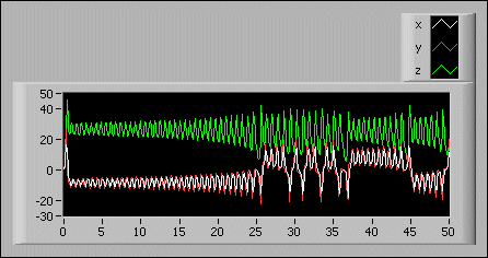
tn ≥ time end.The following illustration shows the solution of the following system of ordinary differential equations:

Enter the following equations on the front panel:
- time start: 0.00
- time end: 50.00
- X: [x, y, z]
- X0: [1, 1, 1]
- F(X,t): [10*(y - x), x*(28 - z) - y, x*y - (8/3)*z]
Examples
Refer to the following example files included with LabVIEW.
- labview\examples\Mathematics\Differential Equations - ODE\Shooting Method.vi
- labview\examples\Mathematics\Differential Equations - ODE\Process Control Explorer.vi