ODE Linear System Symbolic VI
- Updated2025-07-30
- 3 minute(s) read
Solves an n-dimension linear system of differential equations with a given start condition. The solution is based on the determination of the eigenvalues and eigenvectors of the underlying matrix. The solution is given in symbolic form.
Inputs/Outputs
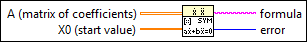
 A (matrix of coefficients)
—
A (matrix of coefficients)
—
A is the n-by-n matrix describing the linear system.  X0 (start value)
—
X0 (start value)
—
X0 is the n vector describing the start condition, x[10], …, x[n0]. There is a one-to-one relation between the components of X0 and X.  formula
—
formula
—
formula is a string with the solution of the linear system in the standard formula notation of LabVIEW. The solution vector elements are separated by carriage return.  error
—
error
—
error returns any error or warning from the VI. Errors are produced by using the wrong inputs X, X0, and F(X,t). You can wire error to the Error Cluster From Error Code VI to convert the error code or warning into an error cluster. |
The linear differential equation described by the following system:

with
x1(0) = 1 x2(0) = 2 x3(0) = 3 x4(0) = 4has the solution
+ 1.62*e(–12.46*t) – 1.28*e(–6.30*t) + 0.63*e(1.34*t) + 0.04*e(5.42*t) + 0.84*e(–12.46*t) – 0.29*e(–6.30*t) + 1.51*e(1.34*t) – 0.06*e(5.42*t) –0.73*e(–12.46*t) + 0.01*e(–6.30*t) + 3.69*e(1.34*t) + 0.02*e(5.42*t) + 0.87*e(–12.46*t) + 2.67*e(–6.30*t) + 0.45*e(1.34*t) + 0.01*e(5.42*t)
The following list of parameters shows how to enter the previous equations on the front panel:
- A: [-7, -6, 4, 1; -6, 2, 1, -2; 4, 1, 0, 2; -1, -2, 2, -7]
- X0: [1, 2, 3, 4]