ODE Linear System Numeric VI
- Updated2026-02-04
- 4 minute(s) read
Requires: Full or Professional Edition
Solves an n-dimension, homogeneous linear system of differential equations with constant coefficients, for a given start condition.
Inputs/Outputs
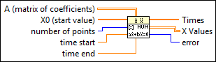
 A (matrix of coefficients)
—
A (matrix of coefficients)
—
A is the n-by-n matrix describing the linear system.  X0 (start value)
—
X0 (start value)
—
X0 is the n vector describing the start condition, x[10], …, x[n0]. There is a one-to-one relation between the components of X0 and X.  number of points
—
number of points
—
number of points is the number of equidistant time points between time start and time end. The default is 10.  time start
—
time start
—
time start is the start point of the ODE. The default is 0.
time end
—
time end is the end point of the time interval under investigation. The default is 1.0.  Times
—
Times
—
Times is an array representing the time steps. The method yields equidistant time steps between time start and time end.  X Values
—
X Values
—
X Values is the matrix of the solution X at the equidistant time points.  error
—
error
—
error returns any error or warning from the VI. Errors are produced by using the wrong inputs X, X0, and F(X,t). You can wire error to the Error Cluster From Error Code VI to convert the error code or warning into an error cluster. |
The solution of the VI is based on the determination of the eigenvalues and eigenvectors of the underlying matrix A. The solution is given in numeric form.
Linear systems can be described by
 X(0) = X0
if time start = 0.
Here
X(t) = (x0(t), …, xn(t))and A represents an n-by-n real matrix. The linear system can be solved by the determination of the eigenvalues and eigenvectors of A. Let S be the set of all eigenvectors spanning the whole n-dimensional space. The transformation Y(t) = SX(t) yields
 Y(0) = SX0
The matrix SAS–1 has diagonal form, so that the solution is obvious. The solution X(t) can be determined by back-transformation
X(t) = S–1Y(t)The following illustration shows the four components of the solution of the linear differential equation described by the following system:

with
x1(0) = 1 x2(0) = 2 x3(0) = 3 x4(0) = 4
The following list of parameters shows how to enter the previous equations on the front panel:
- A: [-7, -6, 4, 1; -6, 2, 1, -2; 4, 1, 0, 2; -1, -2, 2, -7]
- X0: [1, 2, 3, 4]
- time start: 0.00
- time end: 1.00