2D Convolution (CDB) VI
- Updated2025-07-30
- 5 minute(s) read
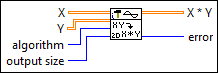
Computes the convolution of the input sequences X and Y. Wire data to the X and Y inputs to determine the polymorphic instance to use or manually select the instance.
Inputs/Outputs
 X
—
X
—
X is the first complex valued input sequence.
Y
—
Y is the second complex valued input sequence.  algorithm
—
algorithm
—
algorithm specifies the convolution method to use. When algorithm is direct, this VI computes the convolution using the direct method of linear convolution. When algorithm is frequency domain, this VI computes the convolution using an FFT-based technique. If X and Y are small, the direct method typically is faster. If X and Y are large, the frequency domain method typically is faster. Additionally, slight numerical differences can exist between the two methods.
output size
—
output size determines the size of X * Y.
 X * Y
—
X * Y
—
X * Y is the convolution of X and Y.  error
—
error
—
error returns any error or warning from the VI. You can wire error to the Error Cluster From Error Code VI to convert the error code or warning into an error cluster. |
2D Convolution
When algorithm is direct, this VI uses the following equation to compute the two-dimensional convolution of the input matrices X and Y.

for i = 0, 1, 2, … , M1+M2–2 and j = 0, 1, 2, … , N1+N2–2
where h is X * Y,
M1 is the number of rows of matrix X, N1 is the number of columns of matrix X, M2 is the number of rows of matrix Y, N2 is the number of columns of matrix Y, The indexed elements outside the ranges of X and Y are equal to zero, as shown in the following relationships:x(m,n), m < 0 or m ≥ M1 or n < 0 or n ≥ N1
and
y(m,n) , m < 0 or m ≥ M2 or n < 0 or n ≥ N2.
When algorithm is frequency domain, this VI completes the following steps, in order, to compute the two-dimensional convolution:
- First, this VI pads the end of X and Y with zeros to make their sizes (M1 + M2 – 1)-by-(N1 + N2 – 2), as shown in the following equations.

- Second, this VI calculates the Fourier transform of X' and Y' according to the following equations.
- Third, this VI multiplies X'(f) by Y'(f) and calculates the inverse Fourier transform of the product. The result is the two-dimensional convolution of X and Y, as shown in the following equation.
The output size determines the size of the output matrix X * Y as shown in the following illustration.

-
full
The output matrix X * Y is (M1+M2–1)-by-(N1+N2–1).
-
size X
This is useful in image processing. If X is the image you want to filter, Y is a small matrix called the convolution kernel. X * Y is the filtered image whose size is the same as that of image X. The output M1-by-N1 matrix is the central part of the output matrix when the output size is full.
-
compact
Computing the edge elements of X * Y requires zero-padding if the output size is full or size X. LabVIEW removes these edge elements if the output size is compact. The output (M1–M2+1)-by-(N1–N2+1) matrix is the central part of the output matrix when the output size is size X.
Examples
Refer to the following example files included with LabVIEW.
- labview\examples\Signal Processing\Signal Operation\Edge Detection with 2D Convolution.vi