1D Convolution (CDB) VI
- Updated2025-07-30
- 4 minute(s) read
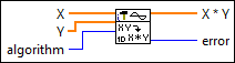
Computes the convolution of the input sequences X and Y. Wire data to the X and Y inputs to determine the polymorphic instance to use or manually select the instance.
Inputs/Outputs
 X
—
X
—
X is the first complex valued input sequence.
Y
—
Y is the second complex valued input sequence.  algorithm
—
algorithm
—
algorithm specifies the convolution method to use. When algorithm is direct, this VI computes the convolution using the direct method of linear convolution. When algorithm is frequency domain, this VI computes the convolution using an FFT-based technique. If X and Y are small, the direct method typically is faster. If X and Y are large, the frequency domain method typically is faster. Additionally, slight numerical differences can exist between the two methods.
 X * Y
—
X * Y
—
X * Y is the convolution of X and Y.  error
—
error
—
error returns any error or warning from the VI. You can wire error to the Error Cluster From Error Code VI to convert the error code or warning into an error cluster. |
1D Convolution
The linear convolution of the signals x(t) and y(t) is defined as:

where the symbol * denotes linear convolution.
When algorithm is direct, this VI uses the following equation to perform the discrete implementation of the linear convolution and obtain the elements of X * Y.

for i = 0, 1, 2, … , M+N–2
where h is X * Y
N is the number of elements in X, M is the number of elements in Y, the indexed elements outside the ranges of X and Y are equal to zero, as shown in the following relationships:xj = 0, j < 0, or j ≥ N
and
yj = 0, j < 0, or j ≥ M.
When algorithm is frequency domain, this VI completes the following steps, in order, to compute the linear convolution:
- First, this VI pads the end of X and Y with zeros to make their lengths M + N – 1, as shown in the following equations.

- Second, this VI calculates the Fourier transform of X' and Y' according to the following equations.
- Third, this VI multiplies X'(f) by Y'(f) and calculates the inverse Fourier transform of the product. The result is the linear convolution of X and Y, as shown in the following equation.
Thus, this VI computes the linear convolution, not the circular convolution. However, because x(t) * y(t)N ⇔ X(f)Y(f) is a Fourier transform pair, where x(t) * y(t)N is the circular convolution of x(t) and y(t), you can create a circular version of the convolution. To compute the circular convolution, you can use a block diagram similar to the block diagram shown in the following illustration.

Examples
Refer to the following example files included with LabVIEW.
- labview\examples\Signal Processing\Signal Operation\Edge Detection with 2D Convolution.vi