Preprocessing a Discrete Time Series (Advanced Signal Processing Toolkit)

Preprocessing helps you make an acquired discrete time series more suitable for further analysis. The LabVIEW Time Series Analysis Tools provide the Preprocessing VIs that enable you to smooth a time series, to resample a time series, or to remove the trend from a time series. The Preprocessing VIs include the Time Series Preprocessing Express VI that you can use to select an appropriate method to preprocess a time series interactively.

Resampling a Time Series

When you acquire a discrete time series, to avoid frequency aliasing, the sampling rate must be greater than twice the highest frequency component of the source signal. If you want to build models for a time series, you usually specify a sampling rate ten times as large as the highest frequency component of the source signal when acquiring the time series. However, a much higher sampling rate substantially increases the computation burden. If the sampling rate is unnecessarily high, you can resample the acquired time series and generate a new time series with a lower sampling rate.

Sometimes the time series under analysis is unequally-sampled. To use time series analysis methods, you need to resample the time series at equal time intervals to generate an equally-sampled time series.

Use the TSA Resampling VI to resample a time series.

Avoiding Frequency Aliasing

Before resampling, the frequency bandwidth of the source signal must be less than the Nyquist frequency at the new sampling rate to avoid aliasing. If the time series contains frequency components whose frequency bands are greater than the new Nyquist frequency, you can use a lowpass filter to attenuate those frequency components that are greater than the new Nyquist frequency.

The following figure shows a time series that contains a frequency component from 100 to 200 Hz and another frequency component from 300 to 400 Hz. The sampling rate of the time series is 1000 Hz.

If the frequency band of interest is from 0 to 250 Hz, you can reduce the sampling rate to 500 Hz. When you resample the time series using the new sampling rate, frequency aliasing occurs if you do not attenuate the frequency component from 300 to 400 Hz because this frequency component is above 250 Hz, the new Nyquist frequency.

The following figure shows the resampled time series that was not properly filtered before resampling and therefore contains frequency aliasing. In the Power Spectrum graph, you can see that frequency aliasing distorts the original frequency component from 100 Hz to 200 Hz.

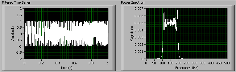
To avoid frequency aliasing in the resampling operation, you first must sufficiently attenuate or filter out the frequency component that is above the new Nyquist frequency. In this example, you need to use a lowpass filter to attenuate the frequency component from 300 to 400 Hz in the original time series.

The following figure shows the filtered time series and the power spectrum. Notice that the lowpass filter removes the frequency component from 300 to 400 Hz from the time series.

After removing the frequency component that is above the new Nyquist frequency, you can resample the time series with the new sampling rate of 500 Hz without frequency aliasing. The following Power Spectrum graph shows that the resampled time series preserves the frequency components of interest from 0 Hz to 250 Hz without distortion.

Converting an Unequally-Sampled Time Series

Time series analysis methods process only equally-sampled time series. To analyze an unequally-sampled time series, you need to convert the unequally-sampled time series into an equally-sampled time series using the TSA Resampling VI.

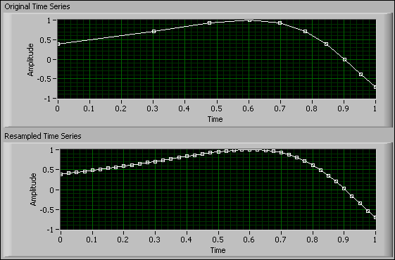
The following figure shows an unequally-sampled time series and the corresponding equally-sampled time series. You can see that the time indexes are distributed equally in the Resampled Time Series graph.

Refer to the Resample Unequally-Sampled Time Series VI in the labview\examples\Time Series Analysis\TSAGettingStarted directory for an example that demonstrates how to convert a unequally-sampled series into an equally-sampled time series with the TSA Resampling VI.

Smoothing a Time Series

Using the Time Series Analysis Tools, you can smooth a time series with either the moving average method or the exponential average method.

The moving average method estimates the local averaged value based on the adjacent values with a finite impulse response (FIR) filter. You can use this method to remove the noise disturbance from a time series.

Use the TSA Moving Average VI to perform a moving average. This VI provides two typical moving average filters—Spencer and Henderson. You also can customize the coefficients of the moving average filters. The TSA Moving Average VI compensates the phase shift of the smoothed time series so no phase delay exists between the original and the smoothed time series.

Exponential averaging is another common approach to producing a smooth time series, which helps you remove the variations that the original time series contains. Exponential averaging also can remove seasonality, which is low-frequency periodic spectral content in a time series.

Use the TSA Exponential Average VI to perform exponential smoothing operations on a time series. You can select a suitable smoothing scheme according to the characteristics of the time series. This VI provides the following exponential smoothing schemes:

• Single exponential smoothing scheme—Suitable for a time series that does not contain a systematic trend or seasonality.
• Double exponential smoothing scheme—Suitable for a time series that contains a systematic trend but does not contain seasonality.
• Triple exponential smoothing scheme—Suitable for a time series that contains both a systematic trend and seasonality.

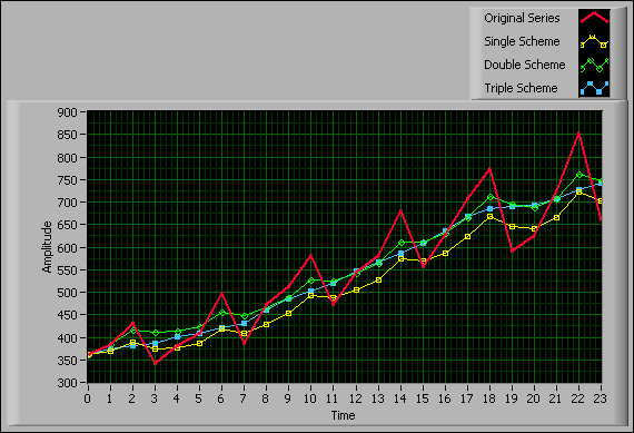
The following figure shows the results of exponential smoothing with different schemes. This figure indicates that the triple scheme follows the time series much closer than the single and double schemes because the time series contains a systematic trend and seasonality.

When using the triple exponential smoothing scheme, you must specify the season type of the analyzed time series. The following figure shows two time series with different types of seasonality—additive and multiplicative.

In the previous figure, the Additive Seasonality graph shows a time series that has a constant amplitude change in seasonality. Using the TSA Exponential Average VI, you can analyze this type of time series by specifying Additive in season type. The Multiplicative Seasonality graph shows a time series that has a seasonality with the amplitude increasing over time. You can analyze this type of time series by specifying Multiplicative in season type.

Detrending a Time Series

A time series usually contains some constant amplitude offset components or low-frequency trends. The constant-offset components and low-frequency trends do not affect the dynamic characteristics of the system being analyzed, and the amplitudes of these trends sometimes are large and corrupt the results of time series modeling. Therefore, you need to remove the constant-offset components or low-frequency trends before performing further analysis.

If a time series contains no long-term (low-frequency) trends but only constant-offset components, you can detrend this time series by subtracting the mean value.

If a time series contains long-term trends and constant-offset components, use the TSA Detrend VI to obtain a detrended time series. This VI estimates the trend of a time series with the curve-fitting methods.