The PID Controller & Theory Explained
Overview
As the name suggests, PID algorithm consists of three basic coefficients; proportional, integral and derivative which are varied to get optimal response. Closed loop systems, the theory of classical PID and the effects of tuning a closed loop control system are discussed in this paper. The PID toolset in LabVIEW and the ease of use of these VIs is also discussed.
Contents
Control System
The basic idea behind a PID controller is to read a sensor, then compute the desired actuator output by calculating proportional, integral, and derivative responses and summing those three components to compute the output. Before we start to define the parameters of a PID controller, we shall see what a closed loop system is and some of the terminologies associated with it.
Closed Loop System
In a typical control system, the process variable is the system parameter that needs to be controlled, such as temperature (ºC), pressure (psi), or flow rate (liters/minute). A sensor is used to measure the process variable and provide feedback to the control system. The set point is the desired or command value for the process variable, such as 100 degrees Celsius in the case of a temperature control system. At any given moment, the difference between the process variable and the set point is used by the control system algorithm (compensator), to determine the desired actuator output to drive the system (plant). For instance, if the measured temperature process variable is 100 ºC and the desired temperature set point is 120 ºC, then the actuator output specified by the control algorithm might be to drive a heater. Driving an actuator to turn on a heater causes the system to become warmer, and results in an increase in the temperature process variable. This is called a closed loop control system, because the process of reading sensors to provide constant feedback and calculating the desired actuator output is repeated continuously and at a fixed loop rate as illustrated in figure 1.
In many cases, the actuator output is not the only signal that has an effect on the system. For instance, in a temperature chamber there might be a source of cool air that sometimes blows into the chamber and disturbs the temperature.Such a term is referred to as disturbance. We usually try to design the control system to minimize the effect of disturbances on the process variable.
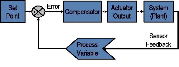
Figure 1: Block diagram of a typical closed loop system.
Defintion of Terminlogies
The control design process begins by defining the performance requirements. Control system performance is often measured by applying a step function as the set point command variable, and then measuring the response of the process variable. Commonly, the response is quantified by measuring defined waveform characteristics. Rise Time is the amount of time the system takes to go from 10% to 90% of the steady-state, or final, value. Percent Overshoot is the amount that the process variable overshoots the final value, expressed as a percentage of the final value. Settling time is the time required for the process variable to settle to within a certain percentage (commonly 5%) of the final value. Steady-State Error is the final difference between the process variable and set point. Note that the exact definition of these quantities will vary in industry and academia.
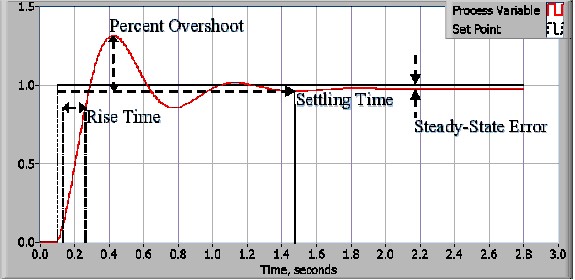
Figure 2: Response of a typical PID closed loop system.
After using one or all of these quantities to define the performance requirements for a control system, it is useful to define the worst case conditions in which the control system will be expected to meet these design requirements. Often times, there is a disturbance in the system that affects the process variable or the measurement of the process variable. It is important to design a control system that performs satisfactorily during worst case conditions. The measure of how well the control system is able to overcome the effects of disturbances is referred to as the disturbance rejection of the control system.
In some cases, the response of the system to a given control output may change over time or in relation to some variable. A nonlinear system is a system in which the control parameters that produce a desired response at one operating point might not produce a satisfactory response at another operating point. For instance, a chamber partially filled with fluid will exhibit a much faster response to heater output when nearly empty than it will when nearly full of fluid. The measure of how well the control system will tolerate disturbances and nonlinearities is referred to as the robustness of the control system.
Some systems exhibit an undesirable behavior called deadtime. Deadtime is a delay between when a process variable changes, and when that change can be observed. For instance, if a temperature sensor is placed far away from a cold water fluid inlet valve, it will not measure a change in temperature immediately if the valve is opened or closed. Deadtime can also be caused by a system or output actuator that is slow to respond to the control command, for instance, a valve that is slow to open or close. A common source of deadtime in chemical plants is the delay caused by the flow of fluid through pipes.
Loop cycle is also an important parameter of a closed loop system. The interval of time between calls to a control algorithm is the loop cycle time. Systems that change quickly or have complex behavior require faster control loop rates.
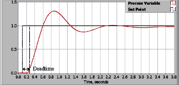
Figure 3: Response of a closed loop system with deadtime.
Once the performance requirements have been specified, it is time to examine the system and select an appropriate control scheme. In the vast majority of applications, a PID control will provide the required results
PID Theory
Proportional Response
The proportional component depends only on the difference between the set point and the process variable. This difference is referred to as the Error term. The proportional gain (Kc) determines the ratio of output response to the error signal. For instance, if the error term has a magnitude of 10, a proportional gain of 5 would produce a proportional response of 50. In general, increasing the proportional gain will increase the speed of the control system response. However, if the proportional gain is too large, the process variable will begin to oscillate. If Kc is increased further, the oscillations will become larger and the system will become unstable and may even oscillate out of control.
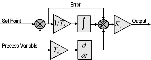
Integral Response
The integral component sums the error term over time. The result is that even a small error term will cause the integral component to increase slowly. The integral response will continually increase over time unless the error is zero, so the effect is to drive the Steady-State error to zero. Steady-State error is the final difference between the process variable and set point. A phenomenon called integral windup results when integral action saturates a controller without the controller driving the error signal toward zero.
Derivative Response
The derivative component causes the output to decrease if the process variable is increasing rapidly. The derivative response is proportional to the rate of change of the process variable. Increasing the derivative time (Td) parameter will cause the control system to react more strongly to changes in the error term and will increase the speed of the overall control system response. Most practical control systems use very small derivative time (Td), because the Derivative Response is highly sensitive to noise in the process variable signal. If the sensor feedback signal is noisy or if the control loop rate is too slow, the derivative response can make the control system unstable
Tuning
The process of setting the optimal gains for P, I and D to get an ideal response from a control system is called tuning. There are different methods of tuning of which the “guess and check” method and the Ziegler Nichols method will be discussed.
The gains of a PID controller can be obtained by trial and error method. Once an engineer understands the significance of each gain parameter, this method becomes relatively easy. In this method, the I and D terms are set to zero first and the proportional gain is increased until the output of the loop oscillates. As one increases the proportional gain, the system becomes faster, but care must be taken not make the system unstable. Once P has been set to obtain a desired fast response, the integral term is increased to stop the oscillations. The integral term reduces the steady state error, but increases overshoot. Some amount of overshoot is always necessary for a fast system so that it could respond to changes immediately. The integral term is tweaked to achieve a minimal steady state error. Once the P and I have been set to get the desired fast control system with minimal steady state error, the derivative term is increased until the loop is acceptably quick to its set point. Increasing derivative term decreases overshoot and yields higher gain with stability but would cause the system to be highly sensitive to noise. Often times, engineers need to tradeoff one characteristic of a control system for another to better meet their requirements.
The Ziegler-Nichols method is another popular method of tuning a PID controller. It is very similar to the trial and error method wherein I and D are set to zero and P is increased until the loop starts to oscillate. Once oscillation starts, the critical gain Kc and the period of oscillations Pc are noted. The P, I and D are then adjusted as per the tabular column shown below.
|
Control
|
P
|
Ti
|
Td
|
|
P
|
0.5Kc
|
-
|
-
|
|
PI
|
0.45Kc
|
Pc/1.2
|
-
|
|
PID
|
0.60Kc
|
0.5Pc
|
Pc/8
|
NI LabVIEW and PID
LabVIEW PID toolset features a wide array of VIs that greatly help in the design of a PID based control system. Control output range limiting, integrator anti-windup and bumpless controller output for PID gain changes are some of the salient features of the PID VI. The PID Advanced VI includes all the features of the PID VI along with non-linear integral action, two degree of freedom control and error-squared control.
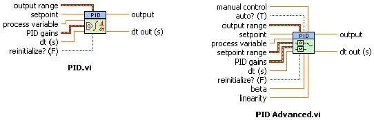
Fig 5: VIs from the PID controls palette of LabVIEW
PID palette also features some advanced VIs like the PID Autotuning VI and the PID Gain Schedule VI. The PID Autotuning VI helps in refining the PID parameters of a control system. Once an educated guess about the values of P, I and D have been made, the PID Autotuning VI helps in refining the PID parameters to obtain better response from the control system.
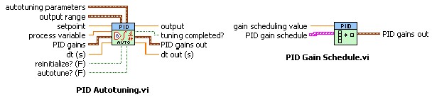
Fig 6: Advanced VIs from the PID controls palette of LabVIEW
The reliability of the controls system is greatly improved by using the LabVIEW Real Time module running on a real time target. NI provides data acquisition devices that provide higher accuracy and better performance than an average control system
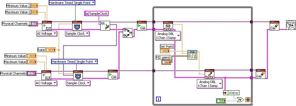
Fig 7: A typical LabVIEW VI showing PID control with a plug-in NI data acquisition device
The tight integration of these data acquisition devices with LabVIEW minimizes the development time involved and greatly increases the productivity of any engineer. Figure 7 shows a typical VI in LabVIEW showing PID control using the NI-DAQmx driver API, which is included with NI data acquisition hardware.
Summary
The PID control algorithm is a robust and simple algorithm that is widely used in the industry. The algorithm has sufficient flexibility to yield excellent results in a wide variety of applications and has been one of the main reasons for the continued use over the years. NI LabVIEW and NI plug-in data acquisition devices offer higher accuracy and better performance to make an excellent PID control system.
References
1. Classical PID Control
by Graham C. Goodwin, Stefan F. Graebe, Mario E. Salgado
Control System Design, Prentice Hall PTR
2. PID Control of Continuous Processes
by John W. Webb Ronald A. Reis
Programmable Logic Controllers, Fourth Edition, Prentice Hall PTR