Sensor Terminology
Overview
This tutorial is part of the NI Measurement Fundamentals series. Each tutorial in this series, will teach you a specific topic of common measurement applications, by explaining the theory and giving practical examples. This tutorial will cover sensors and the terminology associated with them. For the complete list of tutorials, return to the NI Measurement Fundamentals Main page.
Contents
- Sensitivity
- Range
- Precision
- Resolution
- Accuracy
- Offset
- Linearity
- Hysteresis
- Response Time
- Dynamic Linearity
Sensitivity
The sensitivity of the sensor is defined as the slope of the output characteristic curve (DY/DX in Figure 1) or, more generally, the minimum input of physical parameter that will create a detectable output change. In some sensors, the sensitivity is defined as the input parameter change required to produce a standardized output change. In others, it is defined as an output voltage change for a given change in input parameter. For example, a typical blood pressure transducer may have a sensitivity rating of
10 mV/V/mm Hg; that is, there will be a 10-mV output voltage for each volt of excitation potential and each mm Hg of applied pressure.
Sensitivity Error
The sensitivity error (shown as a dotted curve in Figure 1) is a departure from the ideal slope of the characteristic curve. For example, the pressure transducer discussed above may have an actual sensitivity of 7.8 mV/V/mm Hg instead of 10 mV/V/mm Hg.
Range
The range of the sensor is the maximum and minimum values of applied parameter that can be measured. For example, a given pressure sensor may have a range of -400 to +400 mm Hg. Alternatively, the positive and negative ranges often are unequal. For example, a certain medical blood pressure transducer is specified to have a minimum (vacuum) limit of -50 mm Hg (Ymin in Figure 1) and a maximum (pressure) limit of +450 mm Hg (Ymax in Figure 1). This specification is common, incidentally, and is one reason doctors and nurses sometimes destroy blood pressure sensors when attempting to draw blood through an arterial line without being mindful of the position of the fluid stopcocks in the system. A small syringe can exert a tremendous vacuum on a closed system.
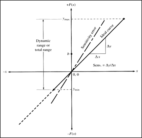
Figure 1. Ideal curve and sensitivity error. Source: J.J. Carr, Sensors and Circuits Prentice Hall.
Dynamic Range
The dynamic range is the total range of the sensor from minimum to maximum. That is, in terms of Figure 1, Rdyn = Ymax - l -Yminl.
Precision
The concept of precision refers to the degree of reproducibility of a measurement. In other words, if exactly the same value were measured a number of times, an ideal sensor would output exactly the same value every time. But real sensors output a range of values distributed in some manner relative to the actual correct value. For example, suppose a pressure of exactly 150 mm Hg is applied to a sensor. Even if the applied pressure never changes, the output values from the sensor will vary considerably. Some subtle problems arise in the matter of precision when the true value and the sensor's mean value are not within a certain distance of each other
(e.g., the 1-s range of the normal distribution curve).
Resolution
This specification is the smallest detectable incremental change of input parameter that can be detected in the output signal. Resolution can be expressed either as a proportion of the reading (or the full-scale reading) or in absolute terms.
Accuracy
The accuracy of the sensor is the maximum difference that will exist between the actual value (which must be measured by a primary or good secondary standard) and the indicated value at the output of the sensor. Again, the accuracy can be expressed either as a percentage of full scale or in absolute terms.
Offset
The offset error of a transducer is defined as the output that will exist when it should be zero or, alternatively, the difference between the actual output value and the specified output value under some particular set of conditions. An example of the first situation in terms of Figure 1 would exist if the characteristic curve had the same sensitivity slope as the ideal but crossed the Y-axis (output) at b instead of zero. An example of the other form of offset is seen in the characteristic curve of a pH electrode shown in Figure 2. The ideal curve will exist only at one temperature (usually 25°C), while the actual curve will be between the minimum temperature and maximum temperature limits depending on the temperature of the sample and electrode.
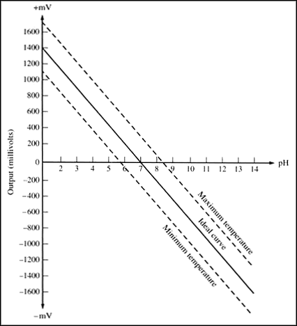
Figure 2. Typical pH electrode characteristic curve showing temperature sensitivity. Source: J.J. Carr, Sensors and Circuits Prentice Hall.
Linearity
The linearity of the transducer is an expression of the extent to which the actual measured curve of a sensor departs from the ideal curve. Figure 3 shows a somewhat exaggerated relationship between the ideal, or least squares fit, line and the actual measured or calibration line (Note in most cases, the static curve is used to determine linearity, and this may deviate somewhat from a dynamic linearity) Linearity is often specified in terms of percentage of nonlinearity, which is defined as:
![]()
where
Nonlinearity (%) is the percentage of nonlinearity
Din(max) is the maximum input deviation
INf.s. is the maximum, full-scale input
The static nonlinearity defined by Equation 6-1 is often subject to environmental factors, including temperature, vibration, acoustic noise level, and humidity. It is important to know under what conditions the specification is valid and departures from those conditions may not yield linear changes of linearity.
Hysteresis
A transducer should be capable of following the changes of the input parameter regardless of which direction the change is made; hysteresis is the measure of this property. Figure 4 shows a typical hysteresis curve. Note that it matters from which direction the change is made. Approaching a fixed input value (point B in Figure 4) from a higher value (point P) will result in a different indication than approaching the same value from a lesser value (point Q or zero). Note that input value B can be represented by F(X)1, F(X)2, or F(X)3 depending on the immediate previous value—clearly an error due to hysteresis.
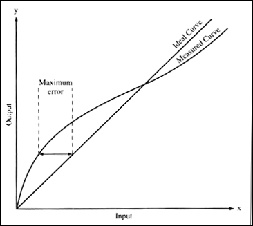
Figure 3. Ideal versus measured curve showing linearity error. Source: J J Carr, Sensors and Circuits Prentice Hall
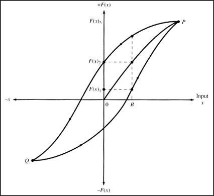
Figure 4. Hysteresis curve. Source: J.J. Carr, Sensors and Circuits Prentice Hall.
Response Time
Sensors do not change output state immediately when an input parameter change occurs. Rather, it will change to the new state over a period of time, called the response time (Tr in Figure 5). The response time can be defined as the time required for a sensor output to change from its previous state to a final settled value within a tolerance band of the correct new value. This concept is somewhat different from the notion of the time constant (T) of the system. This term can be defined in a manner similar to that for a capacitor charging through a resistance and is usually less than the response time.
The curves in Figure 5 show two types of response time. In Figure 5a the curve represents the response time following an abrupt positive going step-function change of the input parameter. The form shown in Figure 5b is a decay time (Td to distinguish from Tr, for they are not always the same) in response to a negative going step-function change of the input parameter.
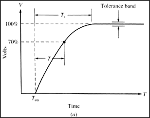
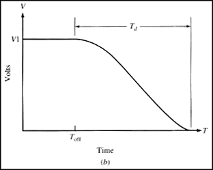
Figure 5. (a) Rise-time definition; (b) fall-time definition. Source: J.J. Carr, Sensors and Circuits Prentice Hall.
Dynamic Linearity
The dynamic linearity of the sensor is a measure of its ability to follow rapid changes in the input parameter. Amplitude distortion characteristics, phase distortion characteristics, and response time are important in determining dynamic linearity. Given a system of low hysteresis (always desirable), the amplitude response is represented by:
+ dX4 + ••• + K (6-2)
In Equation 6-2, the term F(X) is the output signal, while the X terms represent the input parameter and its harmonics, and K is an offset constant (if any). The harmonics become especially important when the error harmonics generated by the sensor action fall into the same frequency bands as the natural harmonics produced by the dynamic action of the input parameter. All continuous waveforms are represented by a Fourier series of a fundamental sinewave and its harmonics. In any nonsinusoidal waveform (including time-varying changes of a physical parameter). Harmonics present will be that can be affected by the action of the sensor.
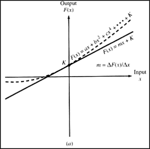

Figure 6. Output versus input signal curves showing (a) quadratic error; (b) cubic error. Source: J.J. Carr, Sensors and Circuits Prentice Hall.
The nature of the nonlinearity of the calibration curve (Figure 6) tell something about which harmonics are present. In Figure 6a, the calibration curve (shown as a dotted line) is asymmetrical, so only odd harmonic terms exist. Assuming a form for the ideal curve of F(x) = mx + K, Equation 6-2 becomes for the symmetrical case:
In the other type of calibration curve (Figure 6b), the indicated values are symmetrical about the ideal mx + K curve. In this case, F(X) = -F(-X), and the form of Equation 6-2 is:
Legal Note
Excerpt from the book, Introduction to Biomedical Equipment Technology, Third Edition, published by Prentice Hall Professional (http://www.phptr.com). Copyright Prentice Hall Inc. 2006. All rights reserved.