Measure Acceleration using a 3-Axis Accelerometer, myDAQ, and LabVIEW

[ExamplePrograms]

Overview

This document explains using a low-cost 3-Axis accelerometer to measure acceleration with your National Instruments myDAQ in LabVIEW. The data will be acquired using the DAQ Assistant that is installed into LabVIEW with the NI DAQmx driver and converted to a temperature using basic programming in LabVIEW.

Objective: 

Use a Freescale MMA7260QT 3-Axis Accelerometer to observe acceleration values with the myDAQ analog input terminals and LabVIEW.

Background:

A 3-Axis accelerometer is very useful in a multitude of applications.  These accelerometers are used to measure G-forces in cars and aircrafts, pedometers, gaming controllers, robotics, and many other applications.  This 3-Axis accelerometer is configured to receive a 3.3VDC input voltage, but the circuitry regulates the voltage down to 3.3 Volts if a supply voltage is greater than 3.3V.  Therefore, we can power the device with the 5V rail on the NI myDAQ.  The sensor then outputs an analog voltage level from 0-3.3VDC, which can be input to the NI myDAQ analog input terminals.  However, the NI myDAQ only has 2 analog inputs, so we will only harness 2-axis of the accelerometer.  Also, this accelerometer has the option to set the sensitivity [g/mV] and input range that can be configured according to the manual that is referenced at the end of this document.

Figure 1: Vishay NTCLE-100E-3103 10kΩ Thermistor

What You Need:

1. NI myDAQ
2. LabVIEW
3. Freescale MMA7260QT 3-Axis Accelerometer from pololu.com ($14.95)
4. Wire
5. Breadboard

Wiring Instructions:

The Accelerometer requires a 5VDC and a Ground input, and it outputs an analog voltage from 0 to 3.3 Volts for each axis, X, Y, and Z.  In this example, we will only use the X- and Y-Axis with the NI myDAQ because there are only 2 differential analog inputs available.  Therefore we will wire the X- and Y-Axis outputs form the sensor to the ai0+ and ai1+ channels, and wire the common ground to the negative terminals of the analog input channels.

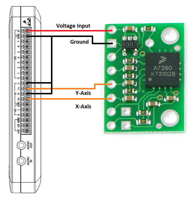
Figure 2: Wiring Diagram

LabVIEW User Interface:

The user interface we created has a numeric control for the sensitivity setting of the accelerometer, a numeric control for the nominal voltage output at zero-g acceleration, and a waveform chart indicator to display the acceleration values.

Figure 3: LabVIEW Front Panel

Coding Strategy:

In LabVIEW, we need to first need to input the analog voltage value from the accelerometer to our NI myDAQ using the DAQ Assistant.  We then need to convert the voltage to an acceleration value using the sensitivity setting for the accelerometer.  Finally we will output the values to a waveform chart on the front panel for the user to view.

Figure 4: Coding Block Diagram

The LabVIEW block diagram looks very similar to the coding block diagram

Figure 5: LabVIEW 2009 Block Diagram

(The attached LabVIEW code snippet can be dragged-and-dropped to a LabVIEW block diagram, use attached PNG file.  After locating the PNG file, just drag the file icon onto a blank block diagram, as if you were dragging the file onto your desktop.)

How It Works:

To understand the application, we must first discuss the configuration of the accelerometer.  By not connecting a digital signal to the g-Select 1 and 2 pins, the default sensitivity for the sensor is 800mV/g, which corresponds to a -1.5g to +1.5g acceleration range.  We can apply a digital True to the pins to change this sensitivity; the maximum range is -6g to +6g with a sensitivity of 200mV/g.  This information can be found on page 4 of the manual, Table 3.  In our application, we will leave these pins unwired, corresponding to a sensitivity of 800mV/g. 

On the block diagram, we will input the data, one point at a time using the DAQ Assistant; the configuration will be discussed in detail below.  We will then read in the value and subtract the nominal zero-g voltage offset as specified in the manual on page 3, Table 2.  The nominal zero-g voltage can be input on the front panel.  Then we can convert the voltage value to an acceleration value by dividing by the sensitivity in V/g.  This sensitivity can be input on the front panel.  This resulting value will be the acceleration in g, from -1.5g to +1.5g, which we can then wire to a waveform chart to display the values on the front panel.  The following steps walk through the configuration of the DAQ Assistant from scratch:

1. Be sure your myDAQ is plugged in
2. Press Ctrl-Space to bring up the Quick Drop Window (takes a full minute to load on the first use)
3. Search for DAQ Assistant and double click on it when it appears in the list
4. Drop it on the Block diagram (white window)
5. When the Create a New Express Task configuration pane appears, select
   1. Acquire Signals
   2. Analog Input
   3. Votlage
   4. Dev 1 (NI myDAQ) *Note: If you have other NI hardware installed, the myDAQ will not be Dev1.
   5. ai0 and ai1 (Use Ctrl+Click for multiple items)
   6. Finish
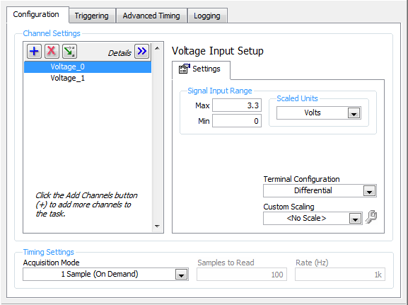
6. Change the Voltage Input Setup to the correct Signal Input Range
   1. Max: 3.3V
   2. Min: 0V
7. Change Timing Settings to
   1. 1 Sample (On Demand)
8. Press OK

Figure 6: DAQ Assistant Voltage Configuration

*Note that sample time is set by the Wait VI and is set to sample 100 times per second (every 10ms) in this VI

Tips and Tricks

• Try to input the acceleration values for duration of one second using a second DAQ Assistant while the accelerometer is experiencing zero-g acceleration.  You can then average these values and use them for the zero-g offset, rather than using the nominal value from the specifications document.
• You can modify the VI to log the data to file using a ‘Write To Spreadsheet File.vi’ express VI if you wish to save the data.  Be sure to place it in the loop and be sure to append new data to the spreadsheet file.
• Expand your application by integrating more logic into the VI.  Possible scenarios might include lighting up an LED when a certain threshold is reached, or create a LED meter that turns on more LEDs as the acceleration increases.  You can use a maximum of 8 LEDs, as demonstrated in the document about the 7-Segment LED indicator.

Related Links

» Freescale MMA7260QT 3-Axis Accelerometer Datasheet

» NI myDAQ Getting Started and Support