From Friday, April 19th (11:00 PM CDT) through Saturday, April 20th (2:00 PM CDT), 2024, ni.com will undergo system upgrades that may result in temporary service interruption.
We appreciate your patience as we improve our online experience.
From Friday, April 19th (11:00 PM CDT) through Saturday, April 20th (2:00 PM CDT), 2024, ni.com will undergo system upgrades that may result in temporary service interruption.
We appreciate your patience as we improve our online experience.
Learn about the time and frequency domain, fast Fourier transforms (FFTs), and windowing as well as how you can use them to improve your understanding of a signal.
The Fourier transform can be powerful in understanding everyday signals and troubleshooting errors in signals. Although the Fourier transform is a complicated mathematical function, it isn’t a complicated concept to understand and relate to your measured signals. Essentially, it takes a signal and breaks it down into sine waves of different amplitudes and frequencies. Let’s take a deeper look at what this means and why it is useful.
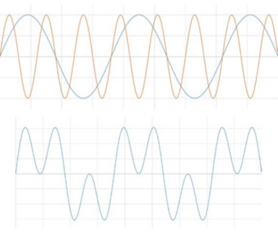
When looking at real-world signals, you usually view them as a voltage changing over time. This is referred to as the time domain. Fourier’s theorem states that any waveform in the time domain can be represented by the weighted sum of sines and cosines. For example, take two sine waves, where one is three times as fast as the other–or the frequency is 1/3 the first signal. When you add them, you can see you get a different signal.
Figure 1: When you add two signals, you get a new signal.
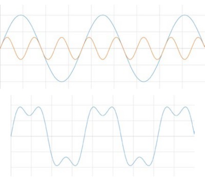
Now imagine if that second wave was also 1/3 the amplitude. This time, just the peaks are affected.
Figure 2: Adjusting the amplitude when adding signals affects the peaks.
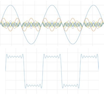
Imagine you added a third signal that was 1/5 the amplitude and frequency of the original signal. If you continued in this fashion until you hit the noise floor, you might recognize the resulting waveform.
Figure 3: A square wave is the sum of sines.
You have now created a square wave. In this way, all signals in the time domain can be represented by a series of sines.
Although it is pretty neat that you can construct signals in this fashion, why do you actually care? Because if you can construct a signal using sines, you can also deconstruct signals into sines. Once a signal is deconstructed, you can then see and analyze the different frequencies that are present in the original signal. Take a look at a few examples where being able to deconstruct a signal has proven useful:
The Fourier transform deconstructs a time domain representation of a signal into the frequency domain representation. The frequency domain shows the voltages present at varying frequencies. It is a different way to look at the same signal.
A digitizer samples a waveform and transforms it into discrete values. Because of this transformation, the Fourier transform will not work on this data. Instead, the discrete Fourier transform (DFT) is used, which produces as its result the frequency domain components in discrete values, or bins. The fast Fourier (FFT) is an optimized implementation of a DFT that takes less computation to perform but essentially just deconstructs a signal.
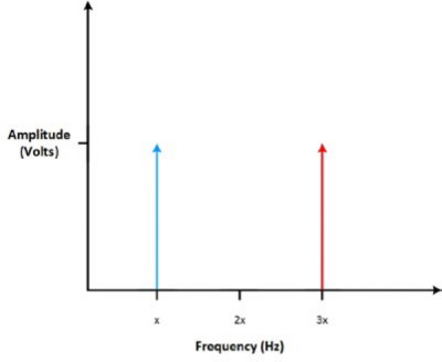
Take a look at the signal from Figure 1 above. There are two signals at two different frequencies; in this case, the signal has two spikes in the frequency domain–one at each of the two frequencies of the sines that composed the signal in the first place.
Figure 4: When two sine waves of equal amplitude are added, they result in two spikes in the frequency domain.
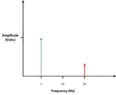
The amplitude of the original signal is represented on the vertical axis. If you look at the signal from Figure 2 above where there are two different signals at different amplitudes, you can see that the most prominent spike corresponds to the frequency of the highest voltage sine signal. Looking at a signal in the time domain, you can get a good idea of the original signal by knowing at what frequencies the largest voltage signals occur.
Figure 5: The highest spike is the frequency of the largest amplitude.
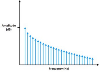
It can also be helpful to look at the shape of the signal in the frequency domain. For instance, let’s take a look at the square wave in the frequency domain. We created the square wave using many sine waves at varying frequencies; as such, you would expect many spikes in the signal in the frequency domain—one for each signal added. If you see a nice ramp in the frequency domain, you know the original signal was a square wave.
Figure 6: The frequency domain of a sine wave looks like a ramp.
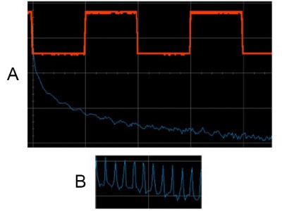
So what does this look like in the real world? Many mixed-signal oscilloscopes (MSO) have an FFT function. Below, you can see what an FFT of a square wave looks like on a mixed-signal graph. If you zoom in, you can actually see the individual spikes in the frequency domain.
Figure 7: The original sine wave and its corresponding FFT are displayed in A, while B is a zoomed in portion of the FFT where you can see the individual spikes.
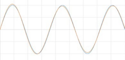
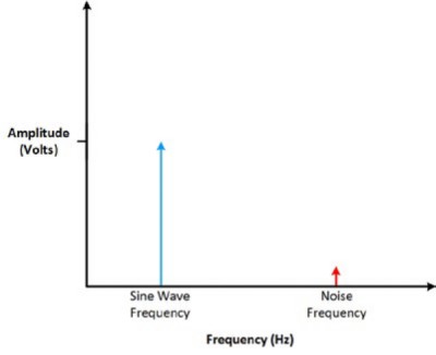
Looking at signals in the frequency domain can help when validating and troubleshooting signals. For instance, say you have a circuit that is supposed to output a sine wave. You can view the output signal on the oscilloscope in the time domain in Figure 8 below. It looks pretty good!
Figure 8: If these two waves were added, they would look like a perfect sine wave because they are so similar.
However, when you view the signal in the frequency domain, you expect only one spike because you are expecting to output a single sine wave at only one frequency. However, you can see that there is a smaller spike at a higher frequency; this is telling you that the sine wave isn’t as good as you thought. You can work with the circuit to eliminate the cause of the noise added at that particular frequency. The frequency domain is great at showing if a clean signal in the time domain actually contains cross talk, noise, or jitter.
Figure 9: Looking at the seemingly perfect sine wave from Figure 8, you can see here that there is actually a glitch.
Although performing an FFT on a signal can provide great insight, it is important to know the limitations of the FFT and how to improve the signal clarity using windowing.
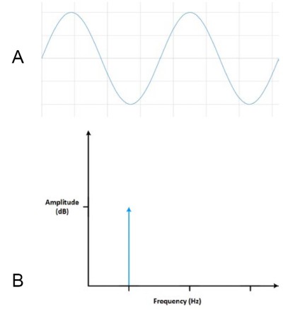
When you use the FFT to measure the frequency component of a signal, you are basing the analysis on a finite set of data. The actual FFT transform assumes that it is a finite data set, a continuous spectrum that is one period of a periodic signal. For the FFT, both the time domain and the frequency domain are circular topologies, so the two endpoints of the time waveform are interpreted as though they were connected together. When the measured signal is periodic and an integer number of periods fill the acquisition time interval, the FFT turns out fine as it matches this assumption.
Figure 10: Measuring an integer number of periods (A) gives an ideal FFT (B).
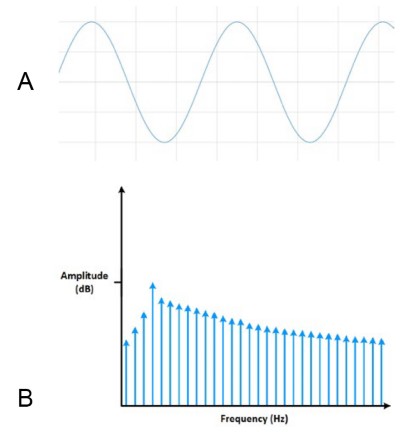
However, many times, the measured signal isn’t an integer number of periods. Therefore, the finiteness of the measured signal may result in a truncated waveform with different characteristics from the original continuous-time signal, and the finiteness can introduce sharp transition changes into the measured signal. The sharp transitions are discontinuities.
When the number of periods in the acquisition is not an integer, the endpoints are discontinuous. These artificial discontinuities show up in the FFT as high-frequency components not present in the original signal. These frequencies can be much higher than the Nyquist frequency and are aliased between 0 and half of your sampling rate. The spectrum you get by using a FFT, therefore, is not the actual spectrum of the original signal, but a smeared version. It appears as if energy at one frequency leaks into other frequencies. This phenomenon is known as spectral leakage, which causes the fine spectral lines to spread into wider signals.
Figure 11: Measuring a noninteger number of periods (A) adds spectral leakage to the FFT (B).
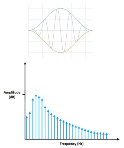
You can minimize the effects of performing an FFT over a noninteger number of cycles by using a technique called windowing. Windowing reduces the amplitude of the discontinuities at the boundaries of each finite sequence acquired by the digitizer. Windowing consists of multiplying the time record by a finite-length window with an amplitude that varies smoothly and gradually toward zero at the edges. This makes the endpoints of the waveform meet and, therefore, results in a continuous waveform without sharp transitions. This technique is also referred to as applying a window.
Figure 12: Applying a window minimizes the effect of spectral leakage.
There are several different types of window functions that you can apply depending on the signal. To understand how a given window affects the frequency spectrum, you need to understand more about the frequency characteristics of windows.
An actual plot of a window shows that the frequency characteristic of a window is a continuous spectrum with a main lobe and several side lobes. The main lobe is centered at each frequency component of the time-domain signal, and the side lobes approach zero. The height of the side lobes indicates the affect the windowing function has on frequencies around main lobes. The side lobe response of a strong sinusoidal signal can overpower the main lobe response of a nearby weak sinusoidal signal. Typically, lower side lobes reduce leakage in the measured FFT but increase the bandwidth of the major lobe. The side lobe roll-off rate is the asymptotic decay rate of the side lobe peaks. By increasing the side lobe roll-off rate, you can reduce spectral leakage.
Selecting a window function is not a simple task. Each window function has its own characteristics and suitability for different applications. To choose a window function, you must estimate the frequency content of the signal.
Even if you use no window, the signal is convolved with a rectangular-shaped window of uniform height, by the nature of taking a snapshot in time of the input signal and working with a discrete signal. This convolution has a sine function characteristic spectrum. For this reason, no window is often called the uniform or rectangular window because there is still a windowing effect.
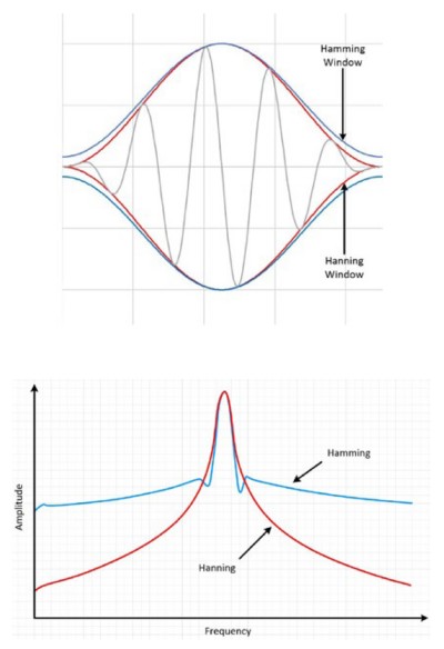
The Hamming and Hann window functions both have a sinusoidal shape. Both windows result in a wide peak but low side lobes. However, the Hann window touches zero at both ends eliminating all discontinuity. The Hamming window doesn’t quite reach zero and thus still has a slight discontinuity in the signal. Because of this difference, the Hamming window does a better job of cancelling the nearest side lobe but a poorer job of canceling any others. These window functions are useful for noise measurements where better frequency resolution than some of the other windows is wanted but moderate side lobes do not present a problem.
Figure 13: Hamming and Hann windowing result in a wide peak but nice low side lobes.
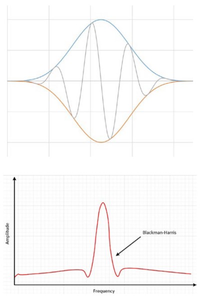
The Blackman-Harris window is similar to Hamming and Hann windows. The resulting spectrum has a wide peak, but good side lobe compression. There are two main types of this window. The 4-term Blackman-Harris is a good general-purpose window, having side lobe rejection in the high 90s dB and a moderately wide main lobe. The 7-term Blackman-Harris window function has all the dynamic range you should ever need, but it comes with a wide main lobe.
Figure 14: The Blackman-Harris results in a wide peak, but good side lobe compression.
A Kaiser-Bessel window strikes a balance among the various conflicting goals of amplitude accuracy, side lobe distance, and side lobe height. It compares roughly to the BlackmanHarris window functions, but for the same main lobe width, the near side lobes tend to be higher, but the further out side lobes are lower. Choosing this window often reveals signals close to the noise floor.
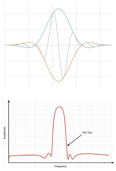
The flat top window is sinusoidal as well, but it actually crosses the zero line. This causes a much broader peak in the frequency domain, which is closer to the true amplitude of the signal than with other windows.
Figure 15: The flat top window results in more accurate amplitude information.
These are just a few of the possible window functions. There is no universal approach for selecting a window function. However, the table below can help you in your initial choice. Always compare the performance of different window functions to find the best one for the application.
| Signal Content | Window |
|---|---|
| Sine wave or combination of sine waves | Hann |
| Sine wave (amplitude accuracy is important) | Flat Top |
| Narrowband random signal (vibration data) | Hann |
| Broadband random (white noise) | Uniform |
| Closely spaced sine waves | Uniform, Hamming |
| Excitation signals (hammer blow) | Force |
| Response signals | Exponential |
| Unknown content | Hann |
| Sine wave or combination of sine waves | Hann |
| Sine wave (amplitude accuracy is important) | Flat Top |
| Narrowband random signal (vibration data) | Hann |
| Broadband random (white noise) | Uniform |
| Two tones with frequencies close but amplitudes very different | Kaiser-Bessel |
| Two tones with frequencies close and almost equal amplitudes | Uniform |
| Accurate single tone amplitude measurements | Flat top |