Top 10 Things to Consider When Choosing an Oscilloscope
Overview
The modern day digital storage oscilloscope is dramatically different from the cathode ray oscilloscope German scientist Karl Ferdinand Braun invented in 1897. Technology advances continue to provide new features that make the oscilloscope more useful to engineers, but one of the most significant transformations of the oscilloscope was its transition into the digital domain, which enabled powerful features such as digital signal processing and waveform analysis. Digital oscilloscopes today include a high-speed, low-resolution (typically 8 bits) analog-to-digital converter (ADC), defined controls and display, and a built-in processor to run software algorithms for common measurements.
Since oscilloscopes are PC-based, you have the advantage of being able to define your instrument functionality in software. As a result, you can use an oscilloscope not only for general measurements, but also for custom measurements, and even as a spectrum analyzer, frequency counter, ultrasonic receiver, or other instrument. With their open architecture and flexible software, oscilloscopes provide several advantages over traditional stand-alone oscilloscopes. When choosing an oscilloscope there are many considerations to keep in mind when selecting the instrument to fit your application.
This paper discusses the top 10 things you should keep in mind if you are considering a new oscilloscope.
Contents
- Bandwidth
- Sampling Rate
- Sampling Modes
- Resolution and Dynamic Range
- Triggering
- Onboard Memory
- Channel Density
- Multiple Instrument Synchronization
- Mixed Signal Capability
- Software, Analysis Capability, and Customizability
- What is the Difference Between an Oscilloscope and a Digitizer?
- Take the Next Step
Bandwidth
Bandwidth describes the frequency range of an input signal that can pass through the analog front end with minimal amplitude loss - from the tip of the probe or test fixture to the input of the ADC. Bandwidth is specified as the frequency at which a sinusoidal input signal is attenuated to 70.7 percent of its original amplitude, also known as the -3 dB point.
In general, it is recommended that you use an oscilloscope with bandwidth at least two times the highest frequency component in your signal.
Oscilloscopes are commonly used for measuring rise time of signals such as digital pulses or other signals with sharp edges. These signals are composed of high-frequency content. To capture the true shape of the signal, you need a high-bandwidth scope. For instance, a 10 MHz square wave is composed of a 10 MHz sine wave and an infinite number of its harmonics. To capture the true shape of this signal, you must use an oscilloscope with bandwidth large enough to capture several of these harmonics. Otherwise, the signal is distorted and your measurements incorrect.
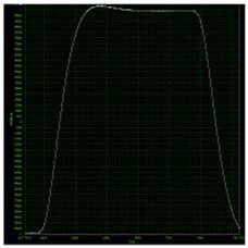
5 MHz square wave acquired with the NI PXI-5152 oscilloscope’s 20 MHz noise filter on.
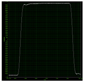
5 MHz square wave acquired with the NI PXI-5152 oscilloscope’s 300 MHz bandwidth
Figure 1: A high-bandwidth scope is important when capturing a waveform with high-frequency components
As a rule of thumb, use the following formula to figure out the bandwidth of your signal based on its rise time (defined as the time taken to transition from 10 to 90 percent of signal amplitude).
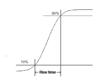
Rise Time = 0.35 / Bandwidth
Figure 2: Rise time defines the time a signal takes to go from 10 to 90 percent of its full-scale value. Rise time and bandwidth are directly related, and one can be calculated from the other using the equation above.
Ideally, you should use a digitizer with three to five times the bandwidth of your signal as calculated in the equation above. In other words, your oscilloscope’s rise time should be 1/5 to 1/3 of your signal’s rise time to acquire your signal with minimal error. You can always backtrack to determine your signal’s real bandwidth based on the following formula:
= measured rise time,
= actual signal rise time,
= oscilloscope’s rise time
Sampling Rate
In the previous section, you learned about bandwidth, which is one of the most important specifications of a oscilloscope. However, high bandwidth can be much less useful if the sample rate is insufficient.
While bandwidth describes the highest frequency sine wave that can be digitized with minimal attenuation, sample rate is simply the rate at which the analog-to-digital converter (ADC) in the oscilloscope is clocked to digitize the incoming signal. Bear in mind that sample rate and bandwidth are not directly related. However, there is a rule of thumb for the desired relationship between these two important specifications:
Oscilloscope real-time sample rate = 3 to 4 times oscilloscope's bandwidth
Nyquist theorem states that to avoid aliasing, the sample rate of a scope needs to be at least twice as fast as the highest frequency component in the signal being measured. However, sampling at just twice the highest frequency component is not enough to accurately reproduce time-domain signals. To accurately digitize the incoming signal, the scopes’s real-time sample rate should be at least three to four times its bandwidth. To understand why, look at the figure below and think about which digitized signal you would rather see on your oscilloscope.
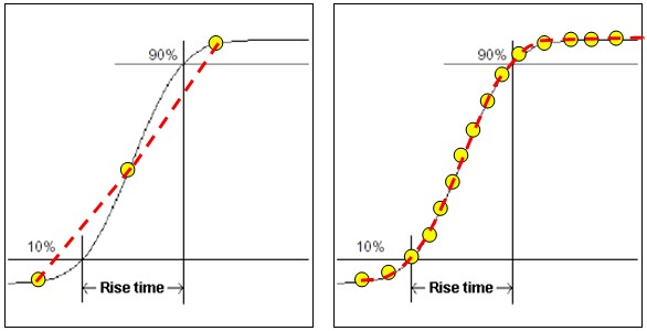
Figure 3: The figure on the right shows a digitizer with a sufficiently high sample rate to accurately reconstruct the signal, which will result in more accurate measurements.
Although the actual signal passed through the front-end analog circuitry is the same in both cases, the image on the left is under sampled, which distorts the digitized signal. On the other hand, the image on the right has enough sample points to accurately reconstruct the signal, which will result in a more accurate measurement. Since a clean representation of the signal is important for time domain applications such as rise time, overshoot, or other pulse measurements, an oscilloscope with a higher sample is beneficial for these applications.
Sampling Modes
There are two main sampling modes – real-time sampling and equivalent-time sampling (ETS).
Real-time sample rate is the one discussed above, which describes the clock rate of the ADC and indicates the maximum rate an incoming signal can be acquired in a single-shot acquisition. On the other hand, equivalent-time sampling is a method of reconstructing a signal based on a series of triggered waveforms that are each acquired in single-shot mode. The advantage of ETS is that it offers a higher effective sample rate. The downside, however, is that it takes more time and is applicable only for repetitive signals. Note that ETS does not increase the oscilloscope’s analog bandwidth, and instead is only useful when you need to reconstruct the signal at a higher sample rate. A common implementation of ETS is random-interleaved sampling (RIS), which is available on most NI oscilloscopes as listed in the table below.
Resolution and Dynamic Range
As described above, digital oscilloscopes have ADCs that convert the signal from analog to digital. The number of bits returned by the ADC is the scope’s resolution. For any given input range, the number of possible discrete levels used to represent the signal digitally is 2b, where b is the resolution. The input range is divided into 2b steps and the smallest possible voltage that is detectable by the oscilloscope is denoted by (Input Range/2b). For example, an 8-bit scope divides a 10 Vpp input range into 28 = 256 levels of 39 mV each, while a 24-bit scope divides the same 10 Vpp input range into 224 = 16,777,216 levels of 596 nV (approximately 65,000 times smaller than in the 8-bit case).
One of the reasons for using a high-resolution oscilloscope is to measure small signals. The question is sometimes asked, why not just use a lower resolution instrument and a smaller range to “zoom in” on the signal to measure small voltages? However, many signals have both a small signal and a large signal component. Using a large range, you could measure the large signal but the tiny signal would be in the noise of the large signal. On the other hand, if you use a small range, then you’d clip the large signal and your measurement would be distorted and invalid. Thus, for applications that involve dynamic signals (signals with large and small voltage components), you need a high-resolution instrument, which has a large dynamic range (the ability of the oscilloscope to measure small signals in the presence of large ones).
Triggering
Typically, oscilloscopes are used to acquire a signal based on a certain event. The instrument’s triggering capability allows you to isolate this event and capture the signal before and after the event. Most oscilloscopes include analog edge, digital, and software triggering. Other triggering options include window, hysteresis, and video triggering.
High-end oscilloscopes feature fast rearm times between triggers, which enables a multi-record capture mode, where the scope captures the specified number of points upon a given trigger, quickly rearms and waits for the next trigger. A fast rearm time ensures that the scope does not miss the event or trigger. Multi-record mode is very useful in capturing and storing only the data that you need, thereby optimizing the use of the onboard memory as well as limiting the activity of the PC bus.
Onboard Memory
Often, data is transferred from the oscilloscope to the PC for measurements and analysis. Although these instruments can sample at their maximum rate, which can be in the several GS/s range, the rate which the data can be transferred to the PC is limited by bandwidth of the connecting bus such as PCI, LAN, GPIB, etc. While today none of these buses can sustain multi-GS/s rates, this may become a non-issue as PCI Express and PXI Express evolve to allow several GB/s data rates.
If the interface bus cannot sustain continuous data transfer at the sample rate of the acquisition, onboard memory on the instrument provides the ability to acquire the signals at the maximum rate and later fetch the data to the PC for processing.
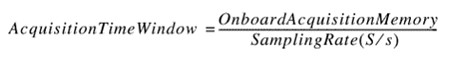
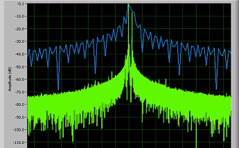
Deep memory not only increases acquisition time, but also provides frequency-domain benefits. The most common frequency-domain measurement is the fast Fourier transform (FFT), which shows a signal’s frequency content. If an FFT has finer frequency resolution, discrete frequencies are more easily detected.
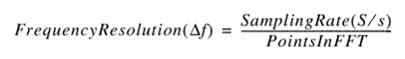
In the equation above, there are two ways to improve the frequency resolution – reduce the sample rate or increase the number of points in the FFT. Reducing the sample rate often is not the ideal solution because this will also reduce your frequency span. In this case, the only solution is to acquire more points for the FFT, which requires deeper onboard memory.
Channel Density
An important factor in an oscilloscope purchasing decision is the number of channels on the instrument or the ability to add channels by synchronizing multiple instruments. Most oscilloscopes have two to four channels, each simultaneously sampled at a certain rate. It is important to be wary of how sample rate is affected when using all the channels. This is because of a commonly used technique called time-interleaved sampling, which interleaves multiple channels to achieve a higher sample rate. If the oscilloscope uses this method and you are using all the channels, you may not be able to acquire at the maximum acquisition rate.
The number of channels required entirely depends on your particular application. Frequently the traditional two to four channels may not be sufficient for a given application, in which case there are two options. The first one is to use a higher channel density product such as the eight-channel (simultaneous) NI PXIe-5105 12-bit, 60 MS/s, 60 MHz oscilloscope. If you are unable to find an instrument that matches your resolution, speed, and bandwidth requirements, you should consider using a platform that lets you scale your test system by providing tight synchronization and allows triggers and clocks to be shared. While it’s practically impossible to synchronize multiple boxed oscilloscopes over GPIB or LAN due to high latency, limited throughput and need for external cabling, PXI provides a superior solution. PXI is an industry standard that adds world-class synchronization technology to existing higher speed busses such as PCI and PCI Express.

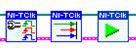
Synchronization of multiple devices is a key requirement of many applications, which can often add to software development time. NI oscilloscopes that are built on the Synchronization and Memory Core (SMC) architecture, however, can make use of NI-TClk to achieve precise synchronization with minimal development effort. NI-TClk provides a high-level interface for programming the synchronization of multiple NI oscilliscopes, arbitrary waveform generators, and high-speed digital I/O devices. Furthermore, there are a variety of prewritten examples for performing this type of synchronization, which makes getting up and running even easier. Shown below are the three functions (niTClk Configure for Homogeneous Triggers, niTClk Synchronize, niTClk Initiate) needed to perform homogenous synchronization on multiple PXI oscilloscopes as programmed in the LabVIEW environment:
Multiple Instrument Synchronization
Almost all automated test and many benchtop applications involve multiple types of instruments such as oscilloscopes, signal generators, digital waveform analyzers, digital waveform generators, and switches.
The inherent timing and synchronization capability of PXI and NI modular instruments allows you to synchronize all these types of instruments without the need for external cabling. For instance, you can integrate a PXI Oscilloscope and a PXI Waveform Generator for performing parameter sweeps, which is useful for characterizing the frequency and phase response of the device under test. The entire sweep can be automated, which obviates the need for manual setting of parameters on the scope and generator followed by offline analysis. A modular approach with PXI results in orders of magnitude improvement in speed and improves your efficiency by letting you focus on the results rather than the cumbersome steps needed to get those results.
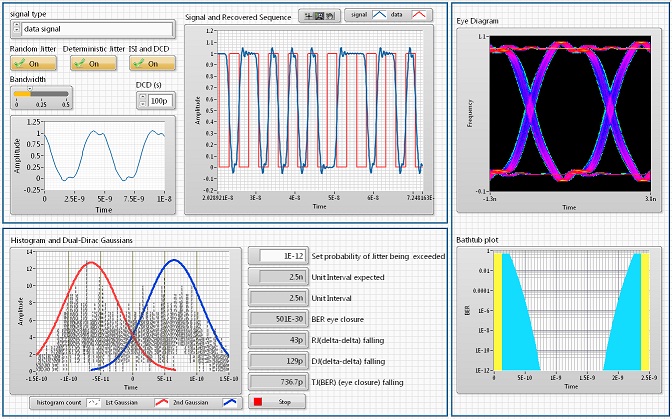
Mixed Signal Capability
The same T-Clk technology that enables creating systems with up to 136 synchronized channels in a single PXI chassis or up to 5000 channels using multiple chassis (as described in the section above) also allows for synchronization of instruments of different types. For instance, an NI oscilloscope can be T-Clk synchronized with signal generators, digital waveform generators, and digital waveform analyzers for building mixed signal systems.
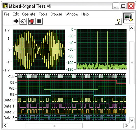
Rather than settle for a mixed-signal oscilloscope with limited digital
functionality, you can use a modular PXI oscilloscope with arbitrary waveform
generators and digital waveform generator/analyzers to build a complete
mixed-signal application with the benefits of both an oscilloscope and a logic
analyzer.
Software, Analysis Capability, and Customizability
Determining software and analysis capabilities is very important when choosing a modular or a stand-alone oscilloscope for your application, and this factor may help you choose between the two instruments.
Stand-alone oscilloscopes are vendor-defined while modular scopes are user-defined and flexible in the applications they can solve. A boxed oscilloscope provides many of the standard functions that are common to the needs of many engineers. As you can imagine, these standard functions will not solve every application, especially for automated test applications. If you need to define the measurements your oscilloscope makes, you might select a modular oscilloscope, which leverages the PC architecture while letting you customize an application to your requirements, instead of the fixed functionality of a stand-alone oscilloscope.
NI oscilloscopes are all programmed using the free NI-SCOPE driver software. This driver comes with more than 50 prewritten example programs that highlight the full functionality of any NI scope, and the included NI-SCOPE Soft Front Panel provides a familiar interface similar to an oscilloscope. The same hardware can also be programmed for both common and custom measurements in a broad range of applications using programming languages including NI LabVIEW, LabWindows/CVI, Visual Basic, and .NET. The driver also supports express configuration-based functions within LabVIEW.
What is the Difference Between an Oscilloscope and a Digitizer?
If you require more customizability than an oscilloscope, such as in-line FPGA processing, a digitizer may be a better fit for your application than an oscilloscope. For example, FlexRIO digitizers also feature high-performance analog-to-digital converters, but allow for more customization. While oscilloscopes are used as general-purpose test equipment, with a flexible front end and selectable input ranges and settings, digitizers are typically used as a more targeted solution for a specific application, for example when designing or prototyping scientific or medical instrumentation.
Unlike modular oscilloscopes, FlexRIO digitizers have fixed analog front-ends, minimal out of the box software functionality, and typical/measured specifications (as opposed to NIST-Certified). However, they are typically available with acquisition speeds and allow for more customization or in-line signal processing via the FPGA.
Take the Next Step
Although both modular and stand-alone oscilloscopes are both used to acquire voltages, the instruments offer different benefits. However, the considerations discussed above are important when purchasing either instrument. Thinking ahead about application requirements, cost constraints, performance, and future expandability can help you choose the instrument that best meets all your needs.