Specifications Explained: NI Multifunction I/O (MIO) DAQ
Overview
Contents
- Introduction
- Understanding Specification Terminology
- Analog Subsystem Specifications
- Digital Subsystem Specifications
- Counter Specifications
- Other Specifications
- Additional Resources
Introduction
This guide is broken up into the same sections as most NI specifications manuals. Terms and definitions below are listed in alphabetical order and may occur in a different order in the specification manuals. This guide exclusively applies to 60xx, 61xx, 62xx, and 63xx families (formerly B, E, S, M, and X Series) MIO DAQ devices and modules. Other NI product families such as cDAQ and cRIO Chassis and Controllers, 91xx, 92xx, 94xx C Series Modules, Multifunction RIO 78xx R Series, Digital Multimeters, Scopes/Digitizers and other instruments may use different terminology or methods to derive specifications and as such, this guide should not be used as a reference for devices and modules other than those in the MIO DAQ family.
This guide will use the NI 6361 and NI 6363 devices as references throughout. If you'd like to follow along with these device specifications, you can do so by following this link: NI 6361 and NI 6363 Specifications.
Understanding Specification Terminology
First, it is important to note the categorical difference between various specifications. NI defines the capabilities and performance of its Test & Measurement instruments as either Specifications, Typical Specifications, and Characteristic or Supplemental Specifications. See your devices' specifications manual for more details on which specifications are warranted or typical.
- Specifications characterize the warranted performance of the instrument within the recommended calibration interval and under the stated operating conditions.
- Typical Specifications are specifications met by the majority of the instruments within the recommended calibration interval and under the stated operating conditions. Typical specifications are not warranted.
- Characteristic or Supplemental Specifications describe basic functions and attributes of the instrument established by design or during development and not evaluated during Verification or Adjustment. They provide information that is relevant for the adequate use of the instrument that is not included in the previous definitions.
Analog Subsystem Specifications
NI MIO DAQ devices and modules may have analog input, analog output, or a mix of both systems. There are specifications unique to each subsystem, but also some specifications which apply to both. This section is organized in three sections to cover the common specifications, analog input specific, and analog output specific.
Analog Input and Analog Output
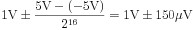
Absolute Accuracy at Full Scale
Accuracy refers to how close to the correct value of a measurement is. Absolute Accuracy at Full Scale is a calculated theoretical accuracy assuming the value being measured is the maximum voltage supported in a given range. The accuracy of a measurement will change as the measurement changes, so to be able to make a comparison between devices, the accuracy at full scale is used. Note that absolute accuracy at full scale makes assumptions about environment variables, such as 25 °C operating temperature, that may be different in practice.
- Nominal Range Positive Full Scale—The ideal maximum positive value that can be measured in a particular range
- Nominal Range Negative Full Scale—The ideal maximum negative value that can be measured in a particular range
- Residual Gain Error—Gain error inherent to the instrumentation amplifier and is known to exist after a self-calibration
- Gain Tempco—The temperature coefficient that describes how temperature impacts the gain of the amplifier compared to the temperature at last self-calibration
- Residual Offset Error—Offset error inherent to the instrumentation amplifier and is known to exist after a self-calibration
- Reference Tempco—The temperature coefficient that describes how accurate a measurement is at a specific temperature compared to the temperature at last external calibration
- INL Error (relative accuracy resolution)—The maximum deviation from the voltage output of an ADC to the ideal output. Can be thought of as worst case DNL. See also: DNL
- Offset Tempco—The temperature coefficient that describes how temperature affects the offset in an ADC conversion compared to the temperature at last self-calibration
- Random/System Noise—Additional system noise generated by the analog front end, measured by grounding the input channel
Example
The NI PXIe-6363 has a range of ± 0.5 V. The absolute accuracy at full scale is calculated with the assumption that the signal being measured is 0.5 V. The absolute accuracy at full scale for the ± 0.5 V range is 100 µV.
See Also
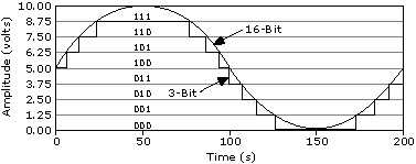
Analog-to-Digital Converter (ADC) Resolution
Resolution is the smallest amount of input signal change that a device or sensor can detect. The number of bits used to represent an analog signal determines the resolution of the ADC.
Example
The NI PXIe-6363 is a 16-bit device, which means that lowest amplitude change that can be detected on the ±5 V range is 0.152 mV. On the ± 0.1 V range, this value is 3.05 µV.
Common Mode Rejection Ratio (CMRR)
When the same signal is seen on the positive and negative inputs of an amplifier, the CMRR specifies how much of this signal is rejected from the final output (typically measured in dB). An ideal amplifier will remove 100% of the common mode signal, but this is not achievable in implementation.
Example
The NI PXIe-6363 has a CMRR of 100 dB. This means that it will attenuate common mode voltages by 100,000x. If the signal being measured is a 5 Vpk sine wave, and the offset or common voltage between the positive and negative inputs is 5 VDC, the final output will reject or attenuate the 5 VDC input to 5 µV. CMRR is not included in accuracy derivations and should be accounted for separately if the signal measured contains common mode voltages.
Convert Interval
The settling time required between channels in a multichannel measurement.
Example
The PCI-6221 has a convert interval ranging from 4 to 7 µs, depending on the level of accuracy required by the user.
See Also
Coupling
A property of the interface of two circuits that defines which types of signals are passed from one side of the interface to the other. There are generally two options:
- DC coupling: will pass both AC and DC signals
- AC coupling: will pass only AC signals, resulting in a hardware implementation of removing a signal's DC offset
Some devices feature software-selectable coupling, while some have either AC or DC.
Example
The NI PXIe-6363 has DC coupling on both the analog input and analog output. It does not support AC coupling on either.
See Also
Crosstalk
The measure of how much a signal on one channel can couple onto, or affect, an adjacent channel. Crosstalk exists any time an amplitude-varying signal is present on a wire or PCB trace that is physically close to another wire or PCB trace.
Example
The NI PXIe-6363 has a crosstalk specification of -75 dB for adjacent channels and -95 dB for non-adjacent channels. This means that channel ai2 will have a crosstalk specification of -75 dB between channels ai1 and ai3, and a crosstalk specification of -95 dB to all other ai channels.
Data Transfer Mechanisms
NI devices bidirectionally transfer data from the device to the computer (in the case of input), and from the computer to the device (in the case of output). Different data transfer mechanism are used depending on the bus (USB, PXI Express, and so on). Some buses can support multiple transfer mechanisms. Refer to the NI-DAQmx help documentation for more information on specific mechanisms.
Example
The USB-6341 supports USB Bulk (Signal Stream) and programmed I/O data transfers. The NI PXIe-6363 supports direct memory access (DMA) and programmed I/O.
See Also
Differential Non-Linearity (DNL)
The difference between the ideal step size of a DAC (See Digital-to-Analog Converter (DAC) Resolution for how to calculate step size) and the actual value that is output (typically measured in LSB). In an ideal DAC, DNL would be 0 LSB.
Example
The NI PXIe-6363 has a DNL of ±1 LSB, which means that for any value that is output from the DAC, the actual value can be ±1 LSB away from the value programmed. For example, if the user programs the DAC to output a value of 1 V on the ±5 V range, the output (not including effects of accuracy) can range from:
INL is the compound effect of DNL so the INL specification is often used in accuracy calculations. For the NI PXIe-6363, the INL specification in the accuracy table is 64 ppm, or 4 LSB, of the range used.
Digital-to-Analog Converter (DAC) Resolution
The number of bits that represents an analog signal when converting from a digital value.
Example
The NI PXIe-6363 uses 16-bit DACs, which means that there are 216 discrete values that can be output in between either ±5 V, ±10 V, or a supplied user voltage.
See Also
Generating a Signal: Types of Function Generators, DAC Considerations, and Other Common Terminology.
FIFO Size (Analog)
NI DAQ devices can store data in an onboard FIFO when performing analog input or analog output tasks.
- For input tasks, this FIFO is used to buffer data prior to the NI-DAQmx driver software transferring the data to a pre-allocated location in RAM known as the PC buffer.
- For output tasks, the data that a user requests to generate can be buffered in a combination of the FIFO and the PC buffer.
Devices that have input and output channels will have a dedicated FIFO for each subsystem. However, the FIFO is shared across all channels within that FIFO. For analog input, NI-DAQmx implements data transfer mechanisms to ensure that the data stored in the FIFO is transferred to the PC buffer fast enough so that the onboard FIFO is not overrun. For analog output, NI-DAQmx implements data transfer mechanisms to ensure that data in the PC buffer is transferred to the onboard FIFO fast enough such that the FIFO is not underrun. For analog output, there are user-selectable properties to specify whether or not to use the PC buffer at all, and to regenerate a single waveform from just the onboard FIFO.
Example
The NI PXIe-6363 has an input FIFO of 2,047 samples. This means that an input task with four channels acquiring data at a rate of 1,024 S/ch/s will overrun the onboard FIFO in less than half a second:

NI-DAQmx uses DMA to transfer data from the FIFO to onboard computer memory, known as the buffer, to avoid the overrun.
See Also
Configuring the Data Transfer Request Condition Property in NI-DAQmx
Waveform Acquisition (DI) FIFO
Waveform Generation (DO) FIFO
Input Bias Current
A consequence of having a finite input impedance is that the device requires a small amount of current to be able to detect a signal. Theoretically, this value should be 0 A, but in practice this is not possible.
Example
The NI PXIe-6363 has an input bias current of ±100 pA. This means that any sensor being measured by the NI PXIe-6363 must be able to source at least that much current across its entire voltage output range in order to be correctly digitized.
Input Current During Overvoltage Condition
When the device is in an overvoltage condition, this is the specified amount of current that the device will sink.
Example
The NI PXIe-6363 sinks a maximum of ±20 mA per pin in an overvoltage state. Exceeding this value may result in damage to critical components.
Input Impedance
Input impedance is a measure of how the input circuitry impedes current from flowing through to analog input ground. For an ideal ADC, this value should be infinite—meaning no current will flow from the input to ground—but in practice this is not possible. The implication of some finite input impedance is that the ADC will have some degree of loading down a circuit, particularly those of high output impedance. It is typical for sensors to have low output impedance.
Example
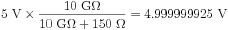
The NI PXIe-6363 has an input impedance of Zin > 10 G Ω. Taking the worst case scenario of lowest input impedance, you can view a single-ended measurement as the following simplified circuit, assuming a sensor with output impedance Zout = 150 Ω.
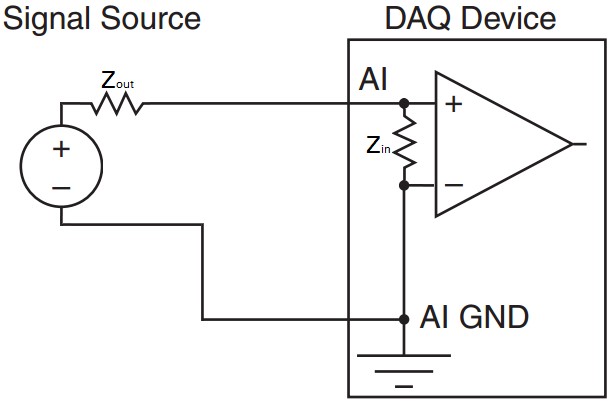
The series combination of the sensor output and DAQ device input means that voltage will be divided between the two impedance values, with the larger impedance bearing most of the voltage. This means that if the sensitivity of this sensor is 20 °C / V and is measuring 100 °C (outputting 5 V), then the voltage measured by the DAQ device will be the output voltage multiplied by the ratio of the input impedance to the sum of the DAQ input and sensor output impedance:
This 75 nV measurement difference corresponds to a near-negligible 05 °C measurement error due to impedance.
To illustrate an example when input impedance becomes an important specification, take the hypothetical case where a sensor has an extremely high output impedance, such as 5 GΩ. Connecting the DAQ device to a sensor with this extremely high output impedance causes a 5 V nominal output from the sensor to be read as 3.33 V, or a hypothetical measurement error of 33.4 °C.
Maximum Update Rate
For analog output, update rate specifies how many samples per second the DAC to analog voltage or current values. Most NI devices have a single DAC per analog output channel, but will all share the FIFO where the analog output data is stored. The rate at which data can be read from this FIFO and transferred to the different DACs on board can sometimes limit the update rate when using multiple AO channels on the same device. Update rate is measured in samples per second (S/s) when outputting from a single channel, or samples per second per channel (S/s/ch) when outputting from multiple channels.
For the analog input equivalent, see Sample Rate.
Example
The NI PXIe-6363 has four analog output channels.
- When using a single channel, the update rate on that channel is 2.86 MS/s.
- When using three channels of analog output, the maximum update rate is 1.54 MS/s/ch—the rate at which data can be read from the FIFO and sent to the various DACs limits the update rate progressively as more channels are added to the scan list.
Maximum Working Voltage
Maximum working voltage specifies the total voltage level that a device can tolerate on any analog input channel before data validity on other channels becomes an issue. The combination of the signal to be measured and any common mode voltage with respect to AI GND should not exceed this maximum working voltage specification to guarantee accuracy on other channels. Note that the maximum working voltage is independent of the input range of the device.
Example
A 10 Vpk sine wave with 2.5 VDC common mode is being measured on a PXIe-6363, which has a maximum working voltage of ± 11 V, as shown below:
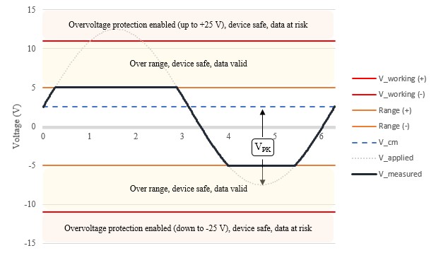
The combination of the two signals peaks at +12.5 V, which exceeds the maximum working voltage. Exceeding the maximum working voltage puts data validity on other multiplexed channels at risk due to excess charge on the multiplexer not having enough time to settle.
See Also
Monotonicity
Monotonicity is the guarantee that when DAC codes increase, the output voltage also increases.
Example
The NI PXIe-6363 guarantees that the output voltage increases as DAC codes increase. For example, a ramp function will always either increase or decrease depending on the direction of the ramp.
Output Current Drive
For analog output, output current drive is the maximum amount of current that the device can sink or source. The load that is connected, including output impedance, combined with the voltage programmed determines the current that will be required to maintain programmed output voltage.
Programmed output voltage is guaranteed if current drive remains below the specified output current drive. Exceeding output current drive puts the device into an overdrive state, where output voltage is no longer guaranteed.
Example
The NI PXIe-6363 is capable of driving ± 5 mA from any analog output channel. On the ± 10 V range, this means that the lowest total impedance that can be driven at full scale is determined from the highest power output, or largest current & voltage:

Taking into account the output impedance of the PXIe-6363, the lowest connected impedance that can be driven at full scale is the difference of the minimum load and the output impedance:

See Also
Output Impedance
Output Impedance is the impedance that is effectively in series with an analog output channel, as illustrated below:
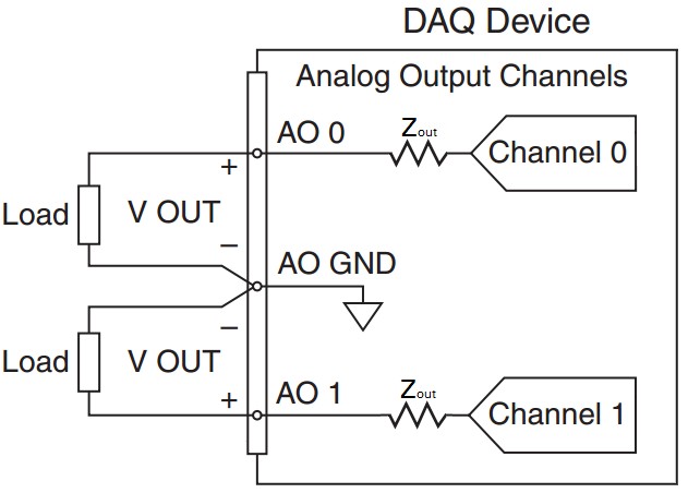
A low output impedance allows more of the voltage generated to be dropped across the load of the analog output. It is important to take the output impedance into account to ensure that the voltage level desired is achieved
Example
The NI PXIe-6363 has an output impedance of 0.2 Ω. This means that if a load connected has an impedance of 500 Ω , and the voltage specified by the user is 1 V, the actual voltage on the load would be 0.9996 V, or 0.4 mV, less than expected. At this voltage, there will also be 1.99 mA drawn from the device.
Overdrive (Short Circuit) Current
If the combination of output and load impedance is too low such that more current is drawn from the device than is specified by the output current drive, the device goes into an overdrive state. Overdrive, or short circuit, current is the maximum amount of current that the device will be able to supply without damage. In this overdrive state, the voltage will droop as current draw increases.
Exceeding the overdrive current may cause damage to the device. NI recommends using the device within the output current drive specification at all times to avoid damaging the device.
Example
The NI 6363 has an overdrive current specification of 26 mA. Exceeding this value, for example during a short circuit, may cause damage to the device.
See Also
Overdrive Protection
For analog output, overdrive protection is the maximum voltage that can be tolerated on the channel before damage to the device occurs. This specification is higher than the actual voltage that can be programmed in the case of accidental back-driven voltage.
Example
The NI PXIe-6363 is protected up to ± 25 V on each analog output channel individually. This means that no matter what voltage is programmed to be output, as long as the voltage at the pin with respect to AO GND is within ± 25 V, no damage will occur to the device. Exceeding this value may cause damage to the device.
Overvoltage Protection
The analog input circuitry has protection diodes in place that will gate a large voltage from damaging the most critical components of the device, such as the PGIA or ADC.
- When the device is powered on, these diodes are biased at some positive and negative voltage, meaning that a voltage larger than the sum of the bias and reverse voltage must be present before these diodes are overloaded and can be damaged.
- When the device is off, the bias voltage is removed, so the voltage needed to reverse the diodes is lower, making the device more susceptible to being damaged.
When in an overvoltage state, the maximum amount of current that a device can sink is specified by the input current during overvoltage condition.
Example
The NI PXIe-6363 has protection up to ±25 V for two AI pins. If more than two AI pins experience an overvoltage larger than ±25 V, the device can be damaged. While the device is off, there is a lower level of protection at ±15 V.
Power-on State
Power-on state specifies the value of an analog output channel when the device has powered on and after a glitching period known as the power-on/off glitch. Prior to the device receiving power from the bus, the value on the output is described in the power-on glitch specification.
Example
The NI PXIe-6363 will have ± 5 mV on the analog output channels upon power-on.
Power-on/off Glitch
When applying and removing power from the device, there is a glitch signal on the analog output channels.
- Glitch Energy Magnitude—The peak amplitude that a glitch signal reaches during a glitch period
- Glitch Energy Duration—The length of time for the glitch signal to subside within the power-on state
Example
The NI PXIe-6363 has a specified glitch of 1.5 Vpk for 200 ms The NI USB-6363 has a specified glitch of 1.5 Vpk for 1.2 s. The glitch period on USB devices can be longer than specified due to firmware updates and USB host performance.
Range (Input or Output)
For analog input, this is the maximum positive and negative value that can be measured with guaranteed accuracy. For analog output, this is the maximum positive or negative value that can be generated. Some devices have multiple input or output ranges that can be used to provide a higher resolution at lower level signals.
Example
The NI PXIe-6363 has four input voltage ranges: ±0.1 V, ±0.2 V, ±0.5 V, ±1 V, ±2 V, ±5 V, ±10 V. It has one output range: ± 10 V.
See Also
Analog-to-Digital Converter (ADC) Resolution
Digital-to-Analog Converter (DAC) Resolution
Sample Rate
Sample rate specifies how often an ADC converts data from analog to digital values. Some devices have only one ADC, so the sample rate is shared across channels while other devices have a dedicated ADC per channel. Sample rate is measured in Samples per second (S/s) or Samples per second per channel (S/s/ch) when acquiring from multiple channels.
- Single Channel Maximum—For a shared sample rate across channels, a single channel can acquire data at a higher rate than allowed when sharing
- Multichannel Maximum—For a device that shares the sample rate across channels, this is the maximum rate at which all channels combined can acquire data
- Minimum—The minimum rate at which data can be acquired
For the analog output equivalent, see Maximum Update Rate.
Example
The NI PXIe-6363 is a multiplexed device, meaning the analog input channels are multiplexed into a single ADC. A single analog input channel can sample analog signals up to 2 million samples per second (2 MS/s). When using multiple channels, the combined rate from all channels must be under 1 MS/s (2 channels can sample at 500 kS/s/ch, 4 channels can sample at 250 kS/s/ch, and so on). There is no minimum sample rate for this device.
Scan List Memory
The number of channels scanned in a task is specified as the scan list memory. An analog input task can contain many virtual channels in a sequence known as a scan list. The scan list can contain the same physical channel many times, and samples may be taken in any arbitrary order. When the task is committed, this scan list is temporarily programmed to the DAQ device.
Example
The NI PXIe-6363 has a scan list memory of 4,095 entries. This means that one scan, or one tick of the sample clock, can trigger up to 4,095 physical channels being read when all physical channels are contained in a single task. However, keeping the settling time for multichannel measurements (also known as convert interval for some devices) in mind, this would limit the sample clock rate to a maximum of around 250 Hz.
Settling Time
The amount of time it takes for an analog output value to stabilize to within a certain degree of precision.
Example
The NI PXIe-6363 has a settling time of a full-scale step to within 1 LSB or 15 ppm of 2 µs. This means that for a full-scale oscillation on the ±5 V range (-5 V, 5 V, -5 V, 5 V, and so on) the maximum frequency that can be driven to within 1 LSB is 1/(2 µs) = 500 kHz.
Settling Time for Multichannel Measurements
The amount of time that the ADC must be connected to each channel when performing a multichannel acquisition.
Example
When acquiring data on the NI PXIe-6363 in a ±10 V range, the multiplexer must remain on a single channel for up to 1.5 µs for the programmable gain instrumentation amplifier (NI-PGIA) to settle within 1 least significant bit (LSB) of the actual value with a full scale step input provided.
Slew Rate
Slew rate specifies the rate of change for the analog output channels in a given device. It is typically measured in V/µs. Settling time for output is calculated with slew time already included in the calculation. It is important to consider slew rate when designing a system for high amplitude high frequency signals, as the large swing in amplitude may exceed the slew rate for a given device.
Example
The NI PXIe-6363 has a typical slew rate of 20 V/µs, this means that the high frequency at full scale that can be generated is 1 MHz. Attempting to output a full scale signal with higher amplitude will result in unwanted distortion.
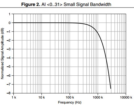
Small Signal Bandwidth
The range of frequencies that is passed with attenuation less than –3 dB. Tests for small signal bandwidth are made with low voltage signals so that slew rate distortion is not a factor.
Example
The NI PXIe-6363 has a small signal bandwidth of 1.7 MHz, as characterized below:
Spurious Free Dynamic Range (SFDR)
Spurious free dynamic range is the usable dynamic range before spurious noise interferes with or distorts the fundamental signal. Analog input and analog output circuitry both have non-linearities that result in harmonic distortion. SFDR is easily observable in the frequency domain as:
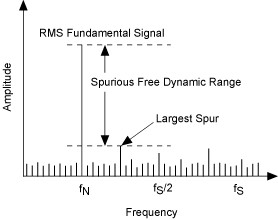
Example
The PCI-6133 has an SFDR of around 95 dB. Taking the graph below as an example, if the fundamental signal was applied at 0 dB, the next highest spur would occur at 95 dB lower - providing a usable dynamic range without spurious interference.
Timing Accuracy
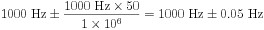
When generating a clock signal on an NI DAQ device for timing signals, the actual frequency generated will be within the timing accuracy. This specification is derived from the overall accuracy of the onboard crystal oscillator. Timing accuracy is typically measured in parts per million (ppm). To convert this accuracy value to Hz, multiply by the accuracy value divided by 1 million. The frequency of the clock is not likely to change drastically from cycle to cycle.
Example
The PXIe-6363 has a timing accuracy of 50 ppm. For an analog output task with an update rate of 1,000 S/s, the sample clock will run at 1,000 Hz ± 50 ppm. In Hz, this comes out to:
Timing Resolution
Sample and update rates for analog input and output tasks are restricted to discrete values when using an onboard timing engine. The difference in clock periods between two adjacent rates is known as timing resolution. NI-DAQmx will coerce a selected frequency up to the next available frequency if it cannot generate the exact one specified by the user.
Example
The NI PXIe-6363 has a specified timing resolution of 10 ns. This means that it can generate or acquire data at integer multiples of 10 ns. For example, 32,000.00 Hz and 32,010.2432... Hz are two adjacent frequencies, as their clock periods are 31.250 µs & 31.240 µs, respectively. To find the next available frequency, add or subtract the timing resolution to a known clock period.
Total Harmonic Distortion (THD)
Due to inherent nonlinearities of ADC and DAC components, harmonic frequencies will appear in the measured or generated signals. The ratio of the sum of these harmonics' powers to the power of the fundamental is known as total harmonic distortion.
Example
The PCI-6133 has a specified THD of around -101 dB. This means that for a given test signal, in this case a 10 kHz sine wave at full scale, the power in the signal attributed to harmonic distortion is less than 0.001%. Conversely, more than 99.999% of the power that is measured can be attributed to the fundamental tone or signal of interest.
Digital Subsystem Specifications
NI MIO DAQ devices and modules may support digital input, digital output, or a mix of both systems. They also support Programmable Function Interface (PFI) lines, which provide a way to route digital signals across the backplane. The following is a list of common specifications, their definition, and how that specification might be used in the real world.
DI Sample Clock frequency
Determines the rate that you can acquire digital waveform data. This specification is different depending on if the device is USB or PCI based (including PCI, PCI Express, PXI, and PXI Express). Typically, PCI based devices will allow for higher digital waveform transfer rates due to the bus' higher sustained throughput, lower latency, and the implementation of direct memory access (DMA) data transfers.
Example
The NI 6363 comes in three form factors: USB, PCI Express, and PXI Express.
- USB - the sample clock frequency can range from 0 to 1 MHz, depending on other devices' activity on the bus. For example, if you are logging data to a USB external hard drive on the same USB hub as your device, you may not be able to achieve the full 1 MHz acquisition rate. For maximum performance, NI recommends that the USB DAQ device is the only device on a USB root hub.
- PCI Express and PXI Express - the sample clock frequency can range from 0 to 10 MHz, depending on other devices' activity on the bus. For example, if a large amount of data is being sent to a GPU for parallel processing during an acquisition, you may not be able to achieve the full 10 MHz acquisition rate. For maximum performance, NI recommends that when a PCI Express or PXI Express device is on the same switch as other devices, that all devices send data in the same direction.
DO Sample Clock frequency
Determines the rate that you can output digital waveform data from port 0 on most NI devices. This specification is different depending on if the device is USB or PCI based (including PCI, PCI Express, PXI, and PXI Express), and where the data is originating from.
- Regenerate from FIFO - A user writes data to the device a single time, and the data is regenerated onboard the device. This method eliminates bus traffic concerns and results in higher output rate.
- Streaming from memory - The device does not regenerate data, so there must always be new data available from the user's application to avoid an underflow error. This method results in constant communication over the bus, therefore update rates are more limited on buses with lower throughput.
Example
The NI 6363 comes in three form factors: USB, PCI Express, and PXI Express.
- USB - Compared with PCI Express and PXI Express, is a lower throughput and higher latency bus. When regenerating an output waveform from the FIFO, the maximum update rate of 10 MHz can be realized. When streaming from memory, data must be streamed over USB, and so a slower maximum rate of 1 MHz is specified.
- PCI Express and PXI Express - These buses are faster and can sustain higher throughput, providing a specified 10 MHz maximum update rate.
Debounce Filter Settings
When a digital line changes state (low-to-high, or high-to-low), it will sometimes bounce between the two states before settling on the new state. A debounce filter can be implemented to ignore the bouncing and only read a value once it has stabilized. For static digital input lines (PFI/Port 1/Port 2) the digital debounce filter is used to debounce noisy or glitchy signals like the kinds that often come from physical interfaces like push buttons. These filters can be customized by the user for any filter length, unlike the digital line filter.
Example
The PXIe-6363 allows for 90 ns, 5.12 µs, 2.56 ms, or custom interval timing for the filter. It also allows programmable high and low transitions as well as being selectable per input line. These filter times are derived from an onboard oscillator on the PXIe-6363.
Delta VT Hysteresis (VT+ - VT-)
Hysteresis is the property of having a different transition threshold depending on whether the value is increasing or decreasing. In this case, the transition observed is from the high to indeterminate state, and low to indeterminate state. The difference between the positive and negative-going threshold is the voltage threshold hysteresis. This specification illustrates how much the voltage level can exceed below or above the threshold before entering the indeterminate state again.
Example
The NI PXIe-6363 specifies a hysteresis of at least 0.2 V. This means that if a signal transitions from 0 to 5 V, it can drop at most 0.2 V below the VT+ value before the logic level may be considered low. During this varying period, the value will cross through the indeterminate state.
Digital Line Filter
When a line filter is enabled on any line in port 0, that line must maintain a stable logic level for the specified filter time in order to be registered as that logic level. This is a helpful tool for transmitting digital data over long cables or in noisy environments. There are typically different filter times that can be selected in software: a short, medium, and long filter. Depending on the characteristics of the noise in your system, one of these filter times may be more appropriate for your application.
Example
The PXIe-6363 has three built-in digital line filter times: 160 ns, 10.24 µs, and 5.12 ms. Note that these filters apply only to lines in port 0. For filtering options on ports 1 and 2, PFI lines, or PXI-specific lines, see Debounce Filter Settings.
Direction Control
Determines whether a digital or PFI line can be configured as an input or output line.
Example
The PXIe-6361 allows each digital or PFI line to be configured as either input or output.
Ground Reference (Digital)
Specifies the reference point where digital signals will be measured or generated with respect to. For example, a logic high digital output may measure 5 volts between the output pin and the specified ground reference.
Example
The PXIe-6361 uses the digital ground (D GND) signal as the ground reference for digital input, digital output, and PFI line signals. Digital ground is separated from analog ground to avoid interference introduced from mixing signals of different level and frequency. Both digital and analog ground are referenced to chassis ground. Extra care should be taken for USB devices, because the analog and digital grounds are referenced to chassis ground of the computer through the USB cable's shield.
Input High Current / Input Low Current (IIH / IIL)
Ideally the input impedance of a device is infinite and no current will be drawn, however this is not achievable in practice. When reading in a digital value at either 0 V or 5 V, a small amount of current will be drawn by the digital input circuitry of the NI device. The amount of current drawn while measuring a high voltage level is input high current, likewise the amount of current drawn while measuring a low voltage level is input low current. It is important to ensure that a digital signal being measured has the capability to tolerate the current values specified.
Example
The NI PXIe-6363 will either source up to 10 µA when Vin = 0 V or sink up to 250 µA when Vin = 5 V. This applies to all digital and PFI lines.
Input High Voltage / Input Low Voltage (VIH / VIL)
The recommended operating voltage ranges that an input signal should be in order to register a logic high or logic low. This specification defines recommended operating conditions so the user knows what values their signal should be, whereas VT+ and VT- are specifications of the device itself.
Example
The NI PXIe-6363 specifies that the voltage input that will get recorded as a low signal ranges from 0 up to 0.8 V. For a high signal, this range is from 2.2 to 5.25 V. Below 0 V and above 5.25 V, the device is in the overvoltage protection state. An indeterminate range also exists where a change from low to high or high to low is not registered until they exceed the VIH or VIL.
See Also
Positive-going Threshold (VT+) / Negative-going Threshold (VT-)
Input Voltage Protection (Digital)
Input Voltage Protection (Digital)
Individual digital input lines have dedicated I/O protection against electrostatic discharge (ESD) and overvoltage conditions. For additional safety of the device, there is a second level of protection that is shared across all digital and PFI lines. Excess overvoltage on multiple lines at the same time stresses this shared protection circuit and may result in damage to the device.
Example
The NI PXIe-6363 has an input voltage protection of ±20 V on up to two pins at the same time. This means that each line individually can handle up to ±20 V in overvoltage safely, but no more than two lines at a time can exceed the nominal voltage input.
See Also
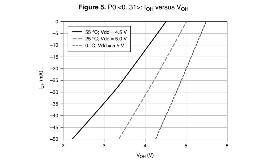
Output High Current / Output Low Current (IOH / IOL)
When outputting a high or a low value, the nominal voltages for most NI devices are 0 and 5 V. However, if a relatively low-impedance load is connected, a higher demand for current is present and this nominal voltage will rise up from 0 V or fall from 5 V. This specification characterises the relationship between the output current and the output voltage.
Example
The PXIe-6363 is capable of sourcing or sinking current depending on if a high value or a low value is written to the pin. For port 0, the maximum recommended value for sourcing and sinking current is 24 mA per line. When current is leaving the device (sourcing) the current is indicated as - 24 mA. When current is entering the device (sinking) the current is indicated as + 24 mA. See the graph below for the characteristic of how much current can be drawn at a given temperature and output voltage.
Port/Sample Size
When acquiring or generating digital waveforms, the number of lines in port 0 define the size of the sample. To limit the amount of traffic on the bus, if a sample contains any combination of lines 0 through 7, the size of the sample will be 1 byte. Similarly, if a sample contains only lines 0 through 15, the size of the sample is reduced to 2 bytes. This follows up to the maximum number of lines in the port, up to the entire size of the port.
Example
The NI PXIe-6363 has 32 lines in port 0. This means that a single digital sample is up to 32 bits (4 bytes) long.
Positive-going Threshold (VT+) / Negative-going Threshold (VT-)
When inputting a logic signal to the device, the value at which a signal will change from the indeterminate range to the logic high range is known as the positive-going threshold. Conversely, the negative-going threshold is the voltage level that must be crossed to register a logic low. The positive-going threshold will always be greater than the negative-going threshold. It is important to ensure that your signal definitively crosses these two levels to accurately register digital states. These specifications refer to the device itself, whereas the input voltage high and low refer to recommended operating conditions.
Example
The NI PXIe-6363 has a VT+ of at most 2.2 V and a VT- of at least 0.8 V.
See Also
Pull-down / Pull-up Resistor
Some NI devices are capable of programatically configuring their digital or PFI lines as input, output, or high impedance. Pull resistors are used to ensure that any pin that would otherwise be floating is referenced to a known signal, such as ground or a voltage source. A pull-down resistor will pull a floating signal to a ground state or logic low, and a pull-up resistor pulls a floating signal to the logic high voltage value.
Example
The PXIe-6361 uses a pull-down resistor of 50 kΩ that ensures terminals not being actively driven high or low will float to a low state.
Waveform Acquisition (DI) FIFO
When reading digital waveform data, there is a temporary storage element onboard the device which buffers the data, known as the FIFO. DAQmx copies data from this FIFO into a block of memory in RAM, known as the PC Buffer. From there, an ADE, such as LabVIEW, copies the data into application memory. The size of this FIFO and the rate that data is being stored in it determine how often the DAQmx driver will copy the data to avoid an overflow condition.
Example
The NI PXIe-6363 has a digital waveform acquisition FIFO of 255 samples. This means that if you are acquiring data at a rate of 100 kbit/s, the onboard FIFO would overflow in about 2.5 ms if the DAQmx driver did not transfer the data in the PC buffer.
Waveform Generation (DO) FIFO
There is temporary storage onboard MIO devices that buffer data points in a first-in-first-out data structure known as the FIFO. This storage is especially useful for USB devices where transfers over the bus take longer, especially when many devices share the same USB root hub. If only a single digital pattern is needed, this pattern can be loaded onto this FIFO to avoid transferring the data over the bus many times. By using the DAQmx API, a user can program for either of these cases.
Example
The NI PXIe-6363 has a digital waveform generation FIFO of 2,047 samples.For example, if you are using the digital output for I2C communication at a data rate of 100 kbit/s, the entire FIFO will be output in 20 ms. This means that the user should call DAQmx Write more frequently than that to continue to stream data to the FIFO. If doing data rate testing, then a single pattern can be loaded into the FIFO using the DAQmx API and output at different data rates without ever having to write new data across the PCI Express bus.
Counter Specifications
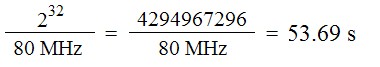
Base Clock Accuracy (general-purpose counters)
The accuracy of an internal base clock directly impacts the accuracy of any measurement or frequency generation from a general-purpose counter. This accuracy is also inherited from the overall device timebase accuracy, meaning that the accuracy of this clock can be improved if a higher accuracy master timebase is externally provided.
Example
The PXIe-6363 has a base clock accuracy of 50 ppm. If a user wants to generate a 12.8 MHz free running clock with this module, the following calculation can be used to determine accuracy:

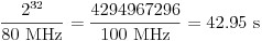
This error can be improved with the use of an external base clock of higher accuracy, or a device with better base clock accuracy, such as the PXIe-6614. The PXIe-6614 uses a more precise and stable oven controlled crystal oscillator (OCXO) that is less susceptible to temperature variation which has a worst case base clock accuracy of 75 ppb. If the same signal was to be generated on this module, the actual frequency would be:

Counter Resolution
The number of bits that a counter can use to represent a number. When a general-purpose counter is configured to output a pulse, the length of time that the pulse is active is represented by the value in the counter's register. The combination of this value and the rate that the counter is counting (set by the counter's base clock) determine the maximum pulse width that can be accomplished. Similarly when using a counter to measure the pulse width of a signal, the maximum pulse width that can be registered is determined by the counter base clock and the resolution of the counter. If a signal exceeds the maximum pulse width the counter will roll over and the NI-DAQmx API will return an error. For this reason, it is important to know how to calculate maximum signal parameters.
Counters with higher resolution provide more flexibility when making the tradeoff between resolution and length of measurements/generations. Refer to the following graph below for more details about this tradeoff.
Example
The PXIe-6614 uses 32-bit counters for counter input and counter output tasks. If a counter input task is configured to measure pulse width, we can calculate the maximum pulse width that can be measured by calculating the maximum counter value and dividing by the counter's internal base clock rate. The 100 MHz counter base clock will allow for 10 ns precision, so that base clock will be selected for this example.
External Base Clock Frequency (general-purpose counters)
If a specific base clock rate is needed, most NI MIO devices allow for the use of an external base clock. This clock serves all the same purposes as an internal base clock, but is externally provided by the user. The maximum rate of an external base clock is dependent on the bus of the device due to bandwidth limitations.
Example
The NI 6363 comes in multiple form factors which have different requirements for an external base clock.
- PCI Express and USB - The frequency range for external base clocks ranges from 0 to 25 MHz, input on any PFI line. The limitation on the maximum frequency is due the bandwidth of a PFI line.
- PXI Express- The PXIe-6363 takes advantage of the advanced capabilities of a PXI Express chassis and allows for up to a 100 MHz signal on the differential star lines (DSTAR).
FIFO (general-purpose counters)
The first-in-first-out (FIFO) memory element onboard MIO devices is used to buffer samples of data for either input or output applications. For counter input applications, data points such as the counter value at specific intervals are stored in the FIFO before DAQmx automatically transfers the data to pre-allocated block of PC RAM. The FIFO is used for counter output applications to store a sequence of duty cycle and frequency values to alter the shape of the waveform being generated. A larger FIFO is useful because it reduces the amount of traffic on the data bus since larger blocks of data can be transferred less frequently than devices with a smaller FIFO.
Example
The PXIe-6614 has a FIFO for each counter that stores 127 samples, allowing for 127 different parameters to be configured for a pulse train generation before additional transfers across the bus are needed.
Internal Base Clocks (general-purpose counters)
The internal base clock for a counter is the signal that will cause the counter's value to increment/decrement depending on the state of the gate terminal. The period of this clock determines the resolution in seconds for a signal being measured or generated but also determines how quickly the counter will roll over when measuring or generating long pulses. For any counter measurement or application, there is a ± 1 timebase period quantization error. To minimize the amount of quantization error, it is important to select the fastest possible base clock for your application.
Example
When performing a measurement using the PXIe-6614 the three internal base clocks that can be used have rates of 100 kHz, 20 MHz, and 100 MHz. These base clocks provide a resolution ranging from 10 µs to 10 ns. If a PWM signal of 125 kHz and 35% duty cycle is applied, the actual pulse width in seconds is 2.8 µs. This is below the resolution of the 100 kHz base clock so it cannot be used for this measurement. The 20 MHz clock has a resolution of 50 ns, so it can perfectly measure the duration of this signal ± 1 base clock pulse. This results in a measurement of 2.8 µs ± 0.05 µs, or an error of about 1.8 %. This same measurement on the 100 MHz clock will result in a measurement of 2.8 µs ± 0.01 µs for an error of 0.36 %. In this case, the 100 MHz clock can measure a pulse width up to about 43 seconds before the counter rolls over, so this pulse width of 2.8 µs is well below the maximum limit.
See Also
Other Specifications
Bus Interface
PCI, PCI Express, PXI, PXI Express, and USB are all examples of bus interfaces that an MIO DAQ device may take. These buses provide some key tradeoffs between data throughput, latency, portability, and channel count.
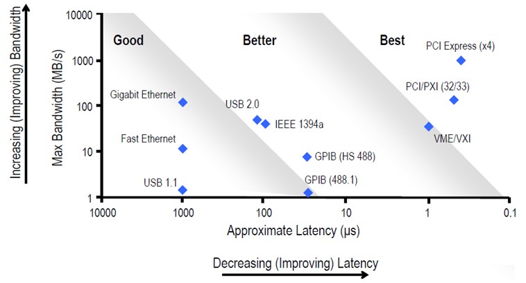
Example
The NI 6363 comes in USB, PXI Express, and PCI Express. While these devices and modules have similar functionality, the PXI Express module and PCI Express device provide lower latency and higher throughput compared to the USB device. The PXI Express module has the additional benefit of the PXI Express system. The USB device has the benefit of being hot-swappable and more compact, making it better for mobile applications.
Calibration
Like all test and measurement equipment, it is important that routine calibration is performed to ensure that the device is operating within the specified accuracy settings. The device has some amount of self-heating, so it is important to allow the specified warm-up time prior to taking any measurements to ensure a stable temperature is reached. At this point, it is recommended that the device is self-calibrated if supported. Refer to Calibration Services for more information about the calibration services that NI offers.
Example
The USB-6363 has a 15 minute warm-up time and a calibration interval of 2 years. NI recommends self-calibrating the device after 15 minutes of being powered on to ensure optimal accuracy. After two years of use, NI recommends sending the device in for a certified calibration.
Current Limits
Every MIO device has a maximum amount of current that it can either sink or source. The specifications in this section are a combination of both sinking and sourcing currents. Some devices have a self resetting fuse on the + 5 V user line in case of accidental surges. Damage to the device can occur if the maximum current specifications are exceeded.
Example
If a PXIe-6363 is driving maximum current from all of its 32 DIO lines on port 0 (24 mA per line), the total current draw from port 0 will be 0.768 A. If there is also a circuit connected to the +5 V user lines on connector 0 and connector 1 that is drawing 0.25 A from each connector, then the module will be supplying a combined 1.268 A. The 0.25 A is within the 1 A max of each power connector, and the 0.768 A draw from the DIO lines combined with the 0.5 A from the + 5 V user lines is within the 2 A maximum of all combined outputs. If this same application were to be used on a PCIe-6363, the optional disk drive connector needs to be connected to ensure that the device operates within the maximum current limits.
Environmental Management
For more information about NI's commitment to design and manufacture products in an environmentally responsible manner, visit Environmental Impact.
External Digital Triggers
MIO devices are capable of importing a digital trigger signal from any PFI line and also exporting some of the most common signals used on the device for synchronization purposes. Signals, such as sample clocks and start triggers, can be output from the MIO device. A digital filter can be applied to any of these signals using the DAQmx API. Refer to your device's routing table in NI MAX for more information about these trigger routes.
- Polarity - indicates whether the signal being exported or imported is active high or active low
Example
The PXIe-6363 is capable of routing the analog input start trigger to any PFI, PXIe_DSTARA, PXIe_DSTARB, PXI_TRIG, or PXI_STAR line that has not yet been reserved for use by another task or device. Looking at the device routes in MAX, this routing is also bidirectional, meaning that the device can accept an analog input start trigger from any of those same sources.
Frequency Generator
In addition to the general purpose counters that exist on MIO devices, there is a separate counter with limited functionality that can be used as a frequency generator. On a typical MIO device, there is a single frequency generator which is limited to a finite number of frequencies that can be generated. The frequencies that can be generated can be used to provide a clock signal to another subsystem on the device, or can be exported for external circuits to use.
Example
The PXIe-6363 has a frequency generator channel that can take one of three base clocks (20 MHz, 10 MHz, and 100 kHz) and divide it down by a divisor from 1 to 16. If a user wants to generate a 50.0 kHz signal, they can select the 100 kHz base clock and a divisor of 2, the following table shows a truncated version of possible frequencies.
| Divisor | Base Clock | ||
|---|---|---|---|
| 20 MHz | 10 MHz | 100 kHz | |
| 1 | 20 MHz | 10 MHz | 100 kHz |
| 2 | 10 MHz | 5 MHz | 50 kHz |
| 3 | 6.67 MHz | 3.33 MHz | 33.3 kHz |
| ... | |||
| 15 | 1.33 MHz | 0.67 MHz | 6.67 kHz |
| 16 | 1.25 MHz | 0.63 MHz | 6.25 kHz |
Operating Temperature
Specifies the ambient temperature range that the MIO device was designed to operate in. This temperature is different than what is reported using the DAQmx API, which is an onboard temperature sensor.
Example
The PXIe-6363 has an operating temperature range of 0 to 55 °C. It is acceptable if the PCB temperature sensor reports higher temperatures during normal use.
Phase-Locked Loop (PLL)
Some MIO devices have a phase-locked loop circuit onboard that allows the device to lock its reference clock to an external reference clock. When a device locks to an external reference clock it inherits the rate, drift, and accuracy of the clock to which it locked. PXI or PXI Express devices automatically lock to the PXI_CLK10 or PXI_CLK100 reference clocks. You can use the NI-DAQmx API to lock to another reference clock source, such as a PFI line.
Example
The USB-6363 has one PLL circuit onboard, and can lock to a 10 MHz clock if present on any PFI line 0 through 15. When configuring a task using the DAQmx API, set the reference clock to the PFI line the external clock is wired into. The PXIe-6363 has a similar PLL circuit, but will automatically lock to the PXI_CLK100 100 MHz clock for synchronization across multiple devices in a PXI Express chassis unless otherwise specified by setting the reference clock source using the DAQmx API. The PCIe-6363 has a PLL circuit that can similarly lock to any PFI or RTSI line. There is no automatic locking on PCI Express or USB devices.
Physical Characteristics
NI publishes dimensional drawings of most products that can be used to check clearance prior to purchasing a device or creating a model of the system being created. In addition to dimensions, NI also provides a comprehensive list of custom cabling, connectors, and screws.
See Also
Dimensional Drawings
NI DAQ Device Custom Cables, Replacement Connectors, and Screws
Power Requirements
It is important to know the power requirements of USB and PCI devices or PXI modules so that the correct amount of power can be sourced. The values indicated in this section are for normal use and do not show the maximum power that a device or module can draw if used outside of specifications. For USB devices, an NI-supplied power supply meets the recommended specifications, but you can use a third party or custom supply if needed. For PCI or PCI Express devices, there is an auxiliary power connector that may be used in case more power is needed. This is most common when using the +5 V user rail for powering an external circuit. Refer to current limits [link to current limits] for more information. For PXI or PXI Express modules, this specification is useful when making a power budget. Refer to the related links for more information.
Example
The PCIe-6363 draws 4.6 W from the +3.3 V rail and 5.4 W from the +12 V rail if the optional disk drive power connector is not installed. The disk drive connector adds a +5 V rail that can supply up to 15 W to the device, while reducing the power draw from the +3.3 V rail to 1.6 W.
See Also
Safety, Electromagnetic Compatibility, CE Compliance
The standards that MIO devices are tested and in compliance with are listed out in the three sections in our specifications manuals. For more information on any standard, visit Product Certifications.
Example
You can view the compliance specifications for the PXIe-6363 by using the certifications search: NI PXIe-6363 - Product Certification
Shock and Vibration
MIO devices are tested to specific industry standards to ensure that stated accuracy according to the specifications and device integrity is maintained over the stated shock and vibration specifications. It is important not to exceed these specified values to ensure correct and accurate operation of the device.
Example
The PCIe-6363 was tested in accordance with IEC 60068-2-27 and the test profile developed in accordance with MIL-PRF-28800F.