Lossless Communication with Network Streams: Components, Architecture, and Performance
Overview
Contents
- Introduction
- About Streams
- Performance Considerations
- Limitations of Network Streams
- Platform Support, Installation, and Configuration
- Benchmarking Data
Introduction
Network streams are an easy-to-configure, tightly integrated, and dynamic communication method for transferring data from one application to another with throughput and latency characteristics that are comparable with TCP. However, unlike TCP, network streams directly support transmission of arbitrary data types without the need to first flatten and unflatten the data into an intermediate data type. Network streams flatten the data in a backwards compatible manner, which enables applications using different versions of the LabVIEW runtime engine to safely and successfully communicate with each other. Network streams also have enhanced connection management that automatically restores network connectivity if a disconnection occurs due to a network outage or other system failure. Streams use a buffered, lossless communication strategy that ensures data written to the stream is never lost, even in environments that have intermittent network connectivity.
Specific Uses
Network streams were designed and optimized for lossless, high throughput data communication. Network streams use a one-way, point-to-point buffered communication model to transmit data between applications. This means that one of the endpoints is the writer of data and the other is the reader. You can accomplish bidirectional communication by using two streams, where each computer contains a reader and a writer that is paired to a writer and reader on the opposite computer.
Because streams were built with throughput characteristics comparable to those of raw TCP, streams are ideal for high throughput applications where the programmer doesn’t want to deal with the complexity of using TCP. Streams can also be used for lossless, low throughput communication such as sending and receiving commands. However, using streams for low throughput communication may require more explicit management over when data is transmitted through the stream if the absolute lowest latency is desired.
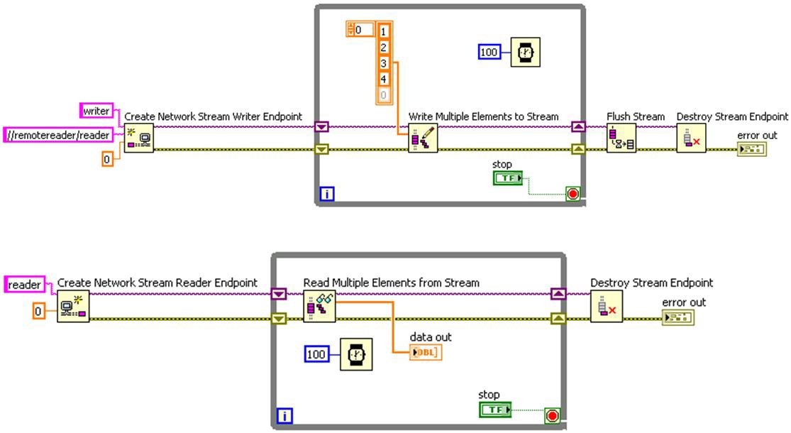
Basic Programming Model
Complete the following steps to create and stream data with a network stream:
1. Create the endpoints and establish the stream connection.
2. Read or write data.
3. Destroy the endpoints.
The following figure shows an implementation of these steps.
About Streams
The following sections describe the details of the general steps outlined in the section above, as well as performance considerations that you should take into account when designing and implementing your application.
Endpoint URLs
LabVIEW identifies each stream endpoint with a URL. To connect two endpoints and create a valid network stream, you must specify the URL of a remote endpoint with the Create Network Stream Endpoint Reader or Create Network Stream Endpoint Writer function. More detailed information on endpoint URLs, including escape codes for reserved characters, can be found in the LabVIEW Help under the topic Specifying Network Stream Endpoint URLs. However, for completeness, a brief description of URLs will be presented here as well.
The full URL of a stream endpoint is as follows:
ni.dex://host_name:context_name/endpoint_name
The following list describes the different components of this URL:
- ni.dex is the protocol of the URL and is optional. If you do not specify ni.dex with the create functions, LabVIEW will infer this protocol.
- host_name is the project alias, DNS name, or IP address of the computer on which the endpoint resides. In addition, the string “localhost” can be used as a pseudonym for the computer on which the code is currently executing. If host_name is left blank, localhost is inferred. LabVIEW searches for a matching host name in the following order: Project alias, DNS name, and then IP address.
- context_name is the name that identifies which application context the endpoint resides in. This is only necessary if the network streams feature is being used by multiple application instances on the same computer. By default, the context name is an empty string and all endpoints are created in the default context. When using the default context, you can omit the colon separator.
- endpoint_name is the actual name of the stream endpoint. This name can be a flat string or a hierarchical path of strings separated by the forward slash character. For example, stream 1 or Subsystem A/stream 1.
The URLs you must specify with the create endpoint functions will vary depending on the network location of the remote machine and the name you assign to the endpoint when you create it.
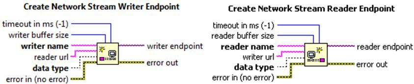
Creating Endpoints and Establishing a Stream
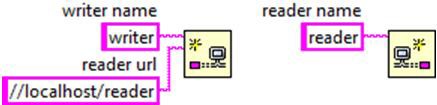
A network stream is the connection between a writer and reader endpoint. You create an endpoint using either the Create Network Stream Writer Endpoint or Create Network Stream Reader Endpoint function.
Creating an endpoint sets several properties on the endpoint that are important when establishing a stream that connects the two endpoints:
- Direction of the endpoint
- Name of the endpoint
- Data type
The direction of the endpoint is implicitly determined by which create function is called and can either be read only or write only. The endpoint name is supplied through the writer name or reader name input to the create function. LabVIEW uses this name to generate a URL for identifying the endpoint resource and must be unique. If an endpoint with the given name already exists, the create function will return an error. The name can be a simple string or a fully compliant URL. Refer to the URL section for more information on what constitutes a valid endpoint URL. While you can connect to existing endpoints that reside on remote machines, you can’t create remote endpoints. You can only create endpoints on the local machine on which the VI is executing.
Unlike TCP, networks streams directly support transmission of LabVIEW data without having to flatten and unflatten the data to and from a string. Most LabVIEW data types are directly supported by network streams. However, a few notable exceptions include data types that contain object references or LabVIEW Classes as part of their type. Classes can still be transferred indirectly by first creating conversion methods on the class to serialize and de-serialize the appropriate class data. Since references are tokens that refer to objects on the local machine, it generally doesn’t make sense to try and send the reference token across the network to be used by a remote computer. The one exception to this is the Vision Image Data Type, which is available if the NI Vision Development Module is installed. In this case, transfer of image data is directly supported by the stream through the use of a reference to the Vision Image Data. Any data types not directly supported by the stream will require conversion code to convert the data to and from one of the supported types. In addition, some data types are more efficient than others to transfer through the stream. See the Performance Considerations section for more information on how the chosen data type can impact the performance of the stream.
In addition to creating the endpoint resources, the create function also links the writer and reader endpoints together to form a fully functioning stream. The endpoint that is created first will wait until the other endpoint has been created and is ready to connect, at which point both create functions will exit. The stream is then ready to transfer data. Used in this manner, the create function effectively acts as a network rendezvous where neither create function will progress until both sides of the stream are ready or until the create call times out.
In order to establish a stream between the two endpoints, three conditions must be satisfied.
1. Both endpoints must exist. In addition, if both create functions specify the remote endpoint URL they are linking against, both URLs must match the endpoints being linked.
2. The data type of the two endpoints must match.
3. One of the endpoints must be a write only endpoint, and the other endpoint must be a read only endpoint.
If condition one isn’t initially satisfied upon executing the create function, it will wait until the timeout expires, and then return a timeout error if the condition still hasn’t been satisfied. If both endpoints specify the other endpoint to link against and only one of the URLs match, one create function will return an error, and the other will continue to wait until the timeout expires.
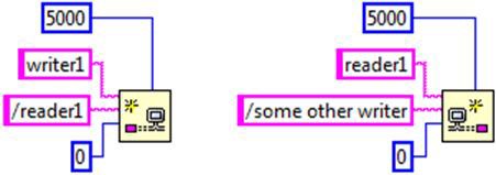
For instance, in the above example, the create call on the left will return an error since the “reader1” endpoint is expecting to communicate with an endpoint named “some other writer” and not “writer1”. However, the create call on the right will continue to wait until the timeout expires for an endpoint named “some other writer” before returning a timeout error. If conditions two or three aren’t met, the create function will return an error as soon as it determines the configuration of the two endpoints isn’t compatible for forming a stream.
When creating endpoints, keep in mind that at least one of the create endpoint functions needs to specify the URL of the other endpoint in either the reader url or writer url input. Failure to do so will guarantee that both create calls will eventually return a timeout error. The reader and writer endpoints can both specify each other’s URLs in their create function, but only one is necessary. In order to develop more portable and maintainable code, National Instruments recommends that only the reader or the writer specify the URL of the other endpoint, but not both.
Endpoint Buffers
Stream endpoints use a FIFO buffer to transfer data from one endpoint to the other. The buffer size is specified at the time of creation, and the buffer is allocated as part of the create call. The size of the buffer is specified in units of elements, where an element in the buffer represents a single value of the type specified by the data type of the stream. Therefore, the total amount of memory consumed by the endpoint will vary depending on the buffer size and the data type of the stream.
For scalar data types like Booleans and numerics, the amount of memory consumed by the endpoint buffer is easy to calculate since the size of a scalar data type is a fixed quantity that is known ahead of time. For instance, a buffer of 1,000 elements of double precision floating point numbers will consume 8,000 bytes of memory since a double precision floating point number always consumes 8 bytes of memory.
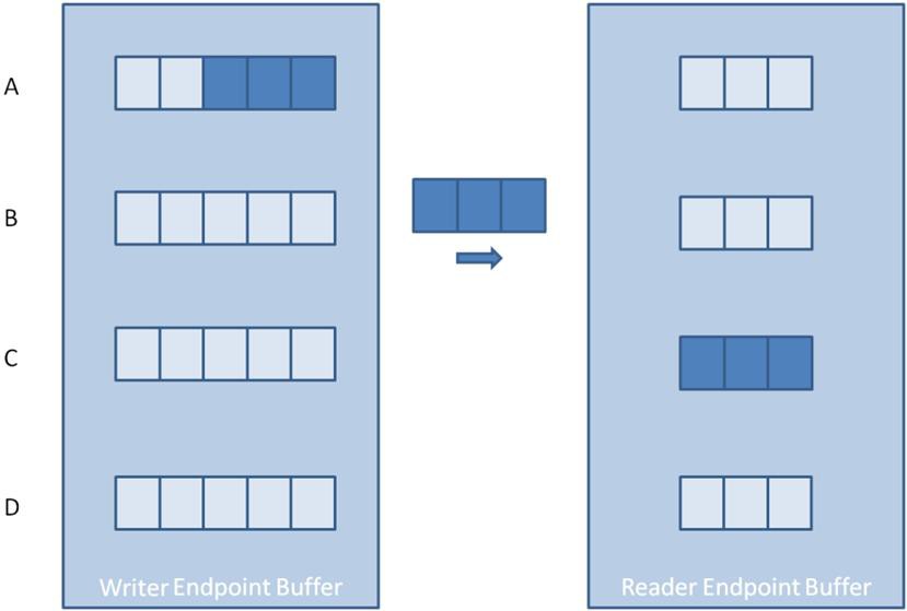
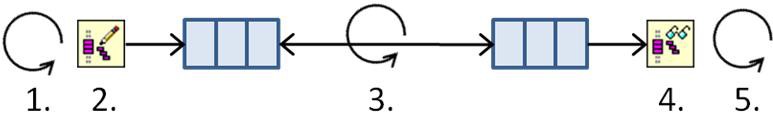
On the other hand, the amount of memory consumed when dealing with non-scalar data types such as clusters, strings, and arrays isn’t as straightforward. The size of these data types can vary at runtime, so the total amount of memory required isn’t known when the endpoint is created. In these cases, the buffer allocated when creating the endpoint is only large enough for each element to hold a pointer or handle to a data value written to that element in the buffer. The memory required to store each element’s data value is then allocated dynamically at runtime as elements are written to the buffer. The image below helps illustrate this concept for a stream endpoint with a buffer size of three and an element data type of 1D array.
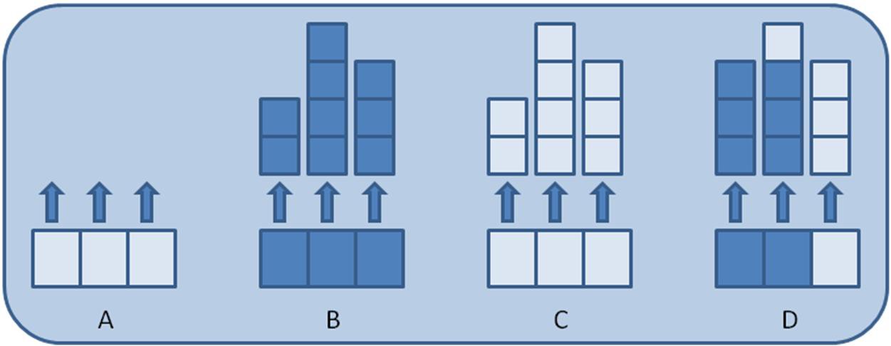
Step A shows the endpoint buffer immediately after creation. At this point, no data values have been written to the endpoint, and each element has been allocated enough memory to store a pointer that will point to the memory block containing the data value for that element.
Step B shows the endpoint buffer after three data values have been written to the buffer. Element 1 contains an array of length two. Element 2 contains an array of length four. Finally, element 3 contains an array of length three. Because this was the first write into the buffer, each write dynamically allocated a block of memory large enough to hold each data value.
Step C shows the endpoint buffer after all three data values have been read from the buffer. Note that even though all values have been read from the buffer, the memory allocated for each data value is not relinquished. Instead, the memory space remains so it can be reused for storing the next data value at that location in the buffer.
Step D shows the endpoint buffer after two more data values of length three have been written. In this case, the memory block maintained by element 1 wasn’t large enough to hold the new data value, and a larger memory block had to be allocated. In contrast, the memory block maintained by element 2 was large enough to hold the new data value and was reused. Notice that even though the memory block maintained by element 2 was larger than needed, it was still reused rather than incurring the execution overhead of de-allocating it and allocating a new block that is of the exact size needed. Once a memory block is allocated for an element, it isn’t relinquished or reduced in size until the endpoint is destroyed.
As this process illustrates, you must choose endpoint buffer sizes carefully for non-scalar data types. If the data elements are large and the buffer size is large, the endpoint may consume large quantities of memory until the endpoint is destroyed. This is also true for scalar data types. However, debugging out of memory issues with scalar data types is typically much easier since all of the required memory is allocated at once when creating the endpoint. In contrast, most of the memory required for non-scalar types is allocated as the buffer is filled for the first time. This can often appear as a memory leak since the application may run successfully for a period of time before running out of memory as the endpoint buffer is filled.
Reading and Writing Data
All read and write calls on the stream are blocking calls that are transactional in nature. They either read or write the requested number of elements successfully, or they time out. In the case of a timeout, no partial data is read or written, and data is never overwritten or regenerated. If a read call results in a timeout, the data out terminal will return the default value for the configured data type. This has the implication that the maximum number of elements that can be read or written in a single call is limited by the endpoint buffer size. A request to read or write a number of elements that is larger than the endpoint buffer size will immediately result in an error.
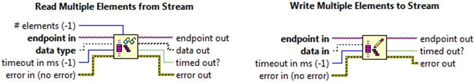
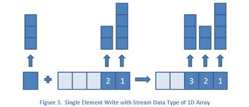
Network streams offer both single element and multiple element interfaces when reading and writing data. Single element reads and writes allow one element at a time to be added or removed from the buffer, while multiple element reads and writes allow data to be added or removed in batches. When using the different types of reads and writes, the representation of the data on the block diagram will be different. In the example below, the data type of the stream is a double precision floating point number. Writing to the stream using the single element write is represented on the block diagram by a data type of double. On the other hand, the data type for the multiple element write data in terminal is represented by an array of doubles.
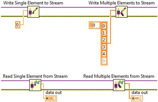
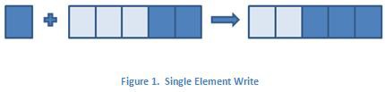
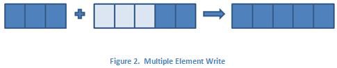
The figures below further illustrate this difference. The elements on the left of the arrow represent the writer endpoint buffer before the write operation occurs, and the elements to the right of the arrow represent the writer endpoint buffer after the write has executed. If the writer endpoint buffer initially has two elements, the execution of the single element write will add one element to the buffer and bring the total number of elements in the buffer to three. If the write multiple elements to stream function is used instead to write three elements, the total number of elements in the buffer will be five.
For non-scalar data types, such as arrays, the figures above look the same, but the contents of the individual elements are array types, which can have varying lengths. In this case, the data type for the single element write is a 1D array, and the data type for the multiple element write is a 2D array. This is illustrated in the figures below where the up arrows and the blocks above them represent the arrays and their respective sizes.
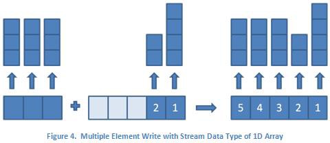
Similarly, the multiple element read will remove as many elements as are specified from the reader endpoint buffer. However, due to the limitations of multi-dimensional array structures in LabVIEW, all of the array elements must have the same dimension lengths. For multiple element reads, this means an error will be returned from the read function if an attempt is made to read multiple elements where the dimension lengths of any of the array elements differ. Using Figure 4 as an example, this means you can successfully read the first element in a single read call, the second element in a single read call, and the third through fifth elements in a single read call. However, any read call that tries to read any combination of the first through third elements will return an error since the dimension lengths of the array elements differ. Since the single and multiple element reads and writes are removing and adding elements from the same buffer, multi-rate applications can mix and match the use of single and multiple element reads and writes as necessary.
When using the multiple elements read function, a value of -1 for the # elements input means read all available samples.
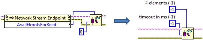
This is equivalent to reading the Available Elements for Reading property and using the returned value as the input for the # elements input to the read function and is a short hand way of accomplishing the same thing. When used in this manner, the timeout in ms input to the read function is effectively disabled. If there are no available elements for reading, the read function will immediately return an empty data array without indicating a timeout or error condition.
Shutting Down a Stream
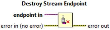
When you no longer need to stream data between the endpoints, you can cease communication from either endpoint by calling the Destroy Stream Endpoint function.
However, if you want to ensure that all data written to the stream has been received by the reader before destroying the writer endpoint, you must first call the Flush Stream function and wait for the appropriate wait condition to be satisfied before destroying the writer endpoint. Only writer endpoints may call the flush function.
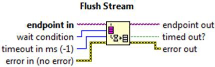
The flush function first requests that any data still residing in the writer endpoint buffer be immediately transferred across the network. It then waits until either the specified wait condition has been met or the timeout expires. The Flush Stream function has two different wait conditions:
- All Elements Read from Stream
- All Elements Available for Reading
When you specify “All Elements Read from Stream,” the flush function will wait until all data has been transferred to the reader endpoint and all data has been read from the reader endpoint before returning. The “All Elements Available for Reading” option will wait until all data has been transferred to the reader endpoint, but it will not wait until all data has been read from the reader endpoint. Using the diagram below as a guide, the “All Elements Available for Reading” option will return from the flush call after step C, and the “All Elements Read from Stream” option will return after step D.
Failure to call flush before destroying the writer endpoint means any data in transit or any data still residing in the writer endpoint buffer could be lost. For this reason, National Instruments recommends that you call flush before shutting down the stream unless your application needs to cease communications immediately and you do not need any data that might be lost in the process.
Once destroy has been called on the reader endpoint, any subsequent write calls from the writer endpoint will result in an error. When the writer endpoint has been destroyed, subsequent read calls from the reader endpoint will continue to succeed until the reader endpoint buffer is empty, at which point, read calls will return errors. If a multiple element read request is received for more elements than remain in the buffer, the read request will return whatever elements are remaining in the buffer, and subsequent read requests will throw an error. This is the only case where a multiple element read request will return fewer points than requested without also indicating a timeout or error condition.
Properties
Network streams have a number of properties available that the application can monitor to obtain information about the ongoing data stream. A few of these properties are explained in more detail below. For information on the remaining properties, see the Network Streams Endpoint Properties page in the LabVIEW help.
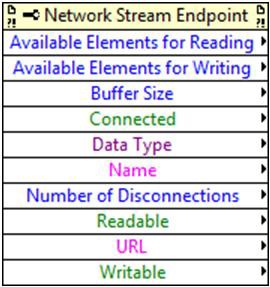
Available Elements for Reading is used by the reader endpoint to return the number of unread elements that reside in the endpoint buffer. This is useful for determining reader endpoint buffer utilization and will only return valid results when read from a reader endpoint. Similarly the “Available Elements for Writing” property returns the number of unwritten elements that reside in the endpoint buffer and can only be read by the writer endpoint. It is often useful to monitor buffer utilization while prototyping applications in order to see how well the reader and writer are keeping up with each other. This information can be used to determine bottlenecks in the application and to fine-tune the endpoint buffer sizes so that the minimum amount of memory resources are consumed while still meeting the overall throughput requirements for the application.
The Connected property indicates the status of the network connection between the reader and writer endpoints. A false on the connected property either indicates that the other endpoint was destroyed using the Destroy Stream Endpoint function or that there is a disruption in the network connection between the two endpoints. In the case of a network disruption, the endpoints will continually try to reconnect in the background until the disruption is resolved or until the endpoint is destroyed.
Number of Disconnections returns the number of times the network connection between the reader and writer endpoints has been disrupted due to problems in the network or from the remote endpoint being destroyed. This property in conjunction with the Connected property can be used to determine the general stability and health of the network connecting reader and writer endpoints.
Lossless Data Transfer and Flow Control
As has been mentioned previously, network streams provide a point-to-point communication channel that preserves all written data until it has been read from the stream or until the stream is destroyed. This lossless data transfer is accomplished through the use of FIFO buffer policies on the endpoint buffers and through acknowledgement and flow control protocol messages. The FIFO buffer policies prevent the application containing the writer endpoint from overwriting data if it’s trying to write data faster than the network can transfer it. The acknowledgement messages prevent data loss from network disconnections, and the flow control messages prevent the application containing the writer endpoint from overwriting data if it’s trying to produce data faster than the application containing the reader endpoint can consume it. The following sequence diagram illustrates in greater detail how these messages are used to ensure lossless data communication.
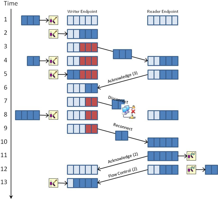
1. Time slot 1 shows a write request of three elements where both endpoint buffers are empty.
2. Because the writer endpoint can accept three elements without overwriting data, the write request completes, and the writer endpoint now contains three elements.
3. The writer endpoint sends three elements to the reader endpoint. At this point, the three elements within the writer endpoint are shaded red to indicate the elements are still occupied pending acknowledgement from the reader endpoint. Until an acknowledgement is received, the writer must hold onto the three elements and can send at most two additional elements.
4. The reader endpoint receives three elements from the writer. A write request of two elements is made on the writer endpoint.
5. The reader endpoint sends an acknowledgement of three elements. Since the writer endpoint can accept two elements without overwriting data, the previous write request from time slot 4 completes, and the writer now contains five elements.
6. The writer endpoint receives an acknowledgement of three elements. It removes three elements from its endpoint buffer, and it now contains two elements.
7. The writer endpoint sends two elements to the reader endpoint. However, in the middle of transmission, there is a network disruption and the data is never received by the reader.
8. A write request of four elements is received. Since the writer endpoint can only accept three elements without overwriting data, the write call blocks.
9. The stream has repaired the network connection and detects that two elements were sent that were never received. These elements are resent as part of the reconnection process.
10. The two resent elements are received by the reader endpoint. The reader now contains five elements and is full. The writer can’t send any more elements until data is read from the reader endpoint.
11. The reader endpoint sends an acknowledgement of two elements. At the same time, a read request for two elements is received.
12. The writer endpoint receives an acknowledgement of two elements and removes them from its endpoint buffer. The writer is now empty. Since the reader has five elements, it completes the previous read request of two elements and sends a flow control message of two elements to the writer endpoint to let it know it can accept an additional two elements without incurring an overflow. The reader now contains three elements.
13. Since the writer now has five free elements, it completes the write request from time slot 8 that has been blocked. The writer now contains four elements. In addition, it receives the flow control message of two elements from the reader. It can now send at most two additional elements to the reader until additional flow control messages are received.
Connection Management and Reconnections
In the previous section we showed how network streams preserve lossless data transfer even in the event of connectivity problems with the underlying network. This section will discuss in more detail how this reconnection process is managed.
In any given network stream, one of the endpoints is designated as the active endpoint, and the other endpoint is designated as the passive endpoint. The active endpoint is the endpoint that originates the initial network connection and is responsible for actively trying to reestablish the connection whenever it detects the network status has become disconnected. Conversely, the passive endpoint is the endpoint that listens or waits to receive a connection request. In terms of client/server terminology, the active endpoint is synonymous with the client, and the passive endpoint is synonymous with the server. The create endpoint function designates which endpoint is the active one. The endpoint that specifies the URL of the remote endpoint it wants to connect to is designated as the active endpoint, and the endpoint that doesn’t specify a URL for the remote endpoint is designated as the passive endpoint.
In the picture above, the writer endpoint on the left is the active endpoint since it specifies the URL of the reader endpoint it’s connecting to. On the other hand, the reader endpoint on the right is designated as the passive endpoint since it doesn’t specify the URL of the endpoint it’s connecting to. If both endpoints specify the remote endpoint they’re connecting to, the endpoint that gets designated as the active endpoint is not deterministic and will depend on the order in which protocol messages are transmitted and received on the network.
In the event of a disconnection, the active endpoint will continuously try to reestablish communication with the passive endpoint in the background. This background process will continue until the connection is repaired or until the endpoint is destroyed. While in the disconnected state, writes to the writer endpoint will continue to succeed until the writer is full, and reads from the reader endpoint will continue to succeed until the reader is empty. Once the writer is full or the reader is empty, read and write calls will block and return timeout indicators as appropriate. However, no errors will be returned from the read or write call itself.
While the endpoint buffers provide some level of protection from jitter due to unreliable networks, they will eventually fill up or empty if the network remains disconnected for too long. If your application needs to tolerate long network outages, you should either size your endpoint buffers to absorb the largest amount of downtime expected or implement appropriate logic to handle timeout conditions in a disconnected state. Also, although a stream is able to recognize it’s in a disconnected state, it can’t always differentiate whether the disconnection is the result of a network problem or an application crash or hang from the application containing the remote endpoint. In the case of a crash or hang, if the endpoint that crashed was the active endpoint, the passive endpoint that is still running will wait forever to receive a reconnection. Since the remote application is no longer responding, this message will never arrive, and the local application will make no further progress with the stream connection. If your application needs to tolerate and recover from crashes or hangs in the remote application, it’s recommended you implement your own watchdog timer by periodically checking the Connected property and taking appropriate action if you are unable to reestablish communication in a reasonable amount of time.
Performance Considerations
Two common metrics when tuning the performance of a network stream are throughput and latency. The measured throughput and latency depend on a number of factors, including the specifications of the systems involved in the communication, the network interface used for the communication, and the overall congestion and reliability of the network itself. While important, detailed discussion of these factors is beyond the scope of this paper. Instead, this paper will focus on properties that are unique to network streams that can be configured programmatically within the application.
Maximizing Throughput
The components that most commonly limit the throughput of a network stream are shown and described below.
1. Writer Application – This is the user application containing the writer endpoint. This will typically involve a loop which calls the Write Function.
2. Write Function – The Write Function represents the cost of accepting the data from the Writer Application and transferring it to the writer endpoint.
3. Network Streams Engine – This is the background process that asynchronously moves data from the writer endpoint to the reader endpoint and sends acknowledgement and flow control messages from the reader endpoint to the writer endpoint.
4. Read Function – The Read Function represents the cost of removing data from the reader endpoint and transferring it to the Reader Application.
5. Reader Application – This is the user application containing the reader endpoint. This will typically involve a loop which calls the Read Function.
Note that the Writer Application, Network Streaming Engine, and Reader Application are all asynchronous processes that run in parallel to each other, and the overall stream throughput will be dictated by the slowest process. Here, the time to execute the Write Function is included as part of the Writer Application, and the time to execute the Read Function is included as part of the Reader Application. A number of streams properties will have an impact on these processes and are discussed in more detail below.
Endpoint Buffer Size
The default buffer size for stream endpoints is 4096 elements. This value tends to be a good compromise between achieving good throughput for scalar data types without consuming huge amounts of memory for non-scalar data types, where the size of each non-scalar element could be very large. While this tends to be a good compromise between throughput and memory utilization for scalar and non-scalar types, it will generally not produce optimal settings for either case. For scalar data types, the endpoint buffer size may need to be on the order of 100,000 or 1,000,000 elements to achieve maximum throughput for a given network interface. For non-scalar types, maximum throughput can often be achieved with much smaller buffers.
Unfortunately, there is no simple formula for determining the optimal buffer size. You will often have to experiment with different buffer sizes during development to determine which settings work best for the needs of your application. As part of the prototyping, you can use the “Available Elements for Reading” and “Available Elements for Writing” properties to determine how effectively each endpoint buffer is being utilized and whether the current buffer size is acting as a bottleneck for the application.
For instance, if you aren’t achieving the desired throughput and the writer endpoint is always full or nearly full, it indicates the Network Streams Engine isn’t keeping up with the Writer Application. This behavior typically signifies that either the network is saturated and has reached its throughput limitations or that the writer endpoint buffer is too small. In the latter case, the network latency for the Network Streams Engine to send elements from the writer endpoint and receive acknowledgement and flow control messages from the reader endpoint is limiting the loop rate of the Writer Application. In this case, you can improve throughput by increasing the writer endpoint buffer size.
Similarly, if you aren’t achieving the desired throughput and the reader endpoint buffer is always empty or nearly empty, it indicates that the Network Streams Engine isn’t keeping up with the Reader Application. This behavior again indicates that the network has reached saturation or that the reader endpoint buffer is too small. Assuming the network hasn’t reached saturation, increasing the reader endpoint buffer size will often improve throughput.
In addition to peak throughput, you should also consider whether or not the stream needs to sustain a minimum average rate of data transfer despite temporary unavailability of the network. For instance, if you’re continuously acquiring 100 kB/s of voltage data from a measurement device, you may find that you only need 10 kB endpoint buffers to sustain the data transfer under ideal conditions. However, if you want to tolerate outages of up to 10 seconds without losing data from your measurement device, you’ll need a minimum writer endpoint buffer size of 1 MB.
Number of Elements to Read and Write
The important thing to remember when reading and writing data is that there is a fixed cost to calling the read or write function regardless of how much data is actually transferred with each read or write call. If you frequently call read or write with relatively small data sets, the total amount of execution time spent on the fixed overhead of the function becomes increasingly significant. If this overhead becomes significant enough, the processor running the Writer Application or Reader Application may become saturated at 100% utilization. When this happens, the processor can no longer execute the application loop fast enough to keep up with the Network Streams Engine, and the application becomes the bottleneck.
To help diagnose this problem, you can look at the endpoint buffer utilization in conjunction with the utilization of the processor running the application. If the processor is near 100% utilization and the writer endpoint is empty or almost always empty, it indicates that the Writer Application isn’t keeping up with the Network Streams Engine. Similarly, if the processor is near 100% utilization and the reader endpoint buffer is full or almost always full, it indicates the Reader Application isn’t keeping up with the Network Streams Engine. In these cases, increasing the number of elements read or written in a single call may improve overall throughput. Alternatively, for variable sized data types, you might try to increase the size of each element written to the stream. For instance, if your element type is a 1D array, you might try writing a single 10,000 element array rather than one thousand 10 element arrays.
Just as reading and writing too little data at a time can be detrimental to throughput, so too can reading and writing too much data at a time. In the case of large data sets, the overhead incurred from paging data into and out of system memory will eventually overtake the overhead saved from calling the read or write function less often. How large the data set can be before this starts to become a limiting factor is system dependent and will vary depending on the amount of physical memory contained by the system. To avoid these issues, a good rule of thumb that works for many applications is to read or write between 1/10th and 1/4th the total buffer size with each read or write call.
Element Data Type
The data type of the stream will also have a direct impact on how much work the read and write functions need to perform in order to flatten and unflatten the data when sending and receiving data across the network. Therefore, more complicated data types will tend to have poorer throughput than simpler data types. The amount of work required to transfer an element of a given data type is determined by the following factors:
1. The complexity and size of the data type itself. For example, arbitrary data types like clusters, which include other data types as sub-elements and can contain arbitrary levels of nesting, are inherently more complicated to parse and construct than data types that have a fixed structure.
2. How efficiently the stream endpoint can manage the memory required to store elements of the data type. If the data type is fixed in size, the endpoint can store all elements in a contiguous block of memory. If the data type is variable sized, the endpoint must manage multiple blocks of memory and occasionally allocate and de-allocate memory at run time.
Based on these criteria, scalar data types are the most efficient and will achieve the best throughput since they’re both simple and fixed in size. Data types that vary in size but are still categorized as simple will have the next best throughput. This class of data type includes arrays of scalars and strings. Finally, data types such as clusters and arrays of clusters that both vary in size and have complex data hierarchies will exhibit the poorest performance. To obtain the highest throughputs, you should strive to use scalar data types whenever possible.
Minimizing Latency
By default, network streams are designed to utilize network bandwidth as efficiently as possible while still maintaining reasonable latency. This means that when data is written to the stream, the stream may hold onto the data for a period of time before transmitting it across the network. This is done so that data from multiple writes in succession can be bundled together and sent as a single large TCP packet across the network rather than a series of smaller packets. The heuristic the stream uses to determine how long to wait before transmitting the data, regardless of how much data is pending, is implementation-dependent and could change from release to release. While this helps to minimize the amount of bandwidth wasted due to TCP packet overhead, it also increases the default latency for low-throughput data streams. If the stream is being used to communicate commands between the two applications, this additional latency may be undesirable. To alleviate this problem, you can call the flush function immediately after the write function, as shown in the figure below.
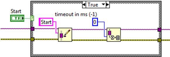
Passing a timeout of zero to the flush function will force the writer endpoint to immediately send all data to the reader endpoint without waiting for the data to be received or read from the reader endpoint. This programming technique will provide the lowest latency possible for sending the data without blocking execution of the writer application.
Limitations of Network Streams
Although networks streams provide a new level of ease of use for conducting point-to-point communication over the network, there are still some situations where network streams may not be a good fit for your application.
In general, network streams are not suitable for use within a control algorithm. Ethernet is typically not a reliable communication bus for control applications, and reads and writes to a stream are not deterministic. Network streams may still be used within the control application to communicate with a remote HMI, but they shouldn’t be used within any time critical loops. Instead, RT FIFOs should be used to send data between the time critical loop and communication loop of the control application. At that point, network streams can be used to exchange data between the communication loops of the control application and remote HMI.
Network streams were designed for lossless, point-to-point communication. While this works well for data streaming and command based applications, it makes establishing arbitrary N:1 or many to many communication paths very difficult. This is a requirement that is common for many client/server applications. Similarly, because streams don’t hold onto the latest value written after it has been read, streams can often be more difficult to use when used for monitoring applications or when updating controls and indicators on an HMI. For these types of applications, other types of communication methods are often more appropriate. For further information on how to choose the right communication methodology for your application, please refer to the tutorial on Using the Right Networking Protocol.
Finally, if the application needs the highest network throughput possible, it may be desirable to use the TCP API instead of network streams. Using TCP will give you the most control over what data is being sent across the network and allow you to customize the communication so that it is optimized for your application. Similarly, if you’re using network streams to communicate between endpoints in the same LabVIEW application context, you may want to consider using Queues for optimal performance. Since the communication is occurring in the same memory context, queues will only use a single memory buffer. This will provide better performance than network streams, which rely on two endpoint buffers regardless of where the endpoints are hosted.
Platform Support, Installation, and Configuration
As of LabVIEW 2010, network streams are only supported on computing targets running Microsoft Windows or LabVIEW Real-Time. For Microsoft Windows, the network streams feature is included as part of the LabVIEW Base version and is available for use immediately upon installation. For information on how to get network streams to work with Windows firewall settings, refer to Knowledge Base 5BCF43RY: Recommended Firewall Settings When Using Network Streams.
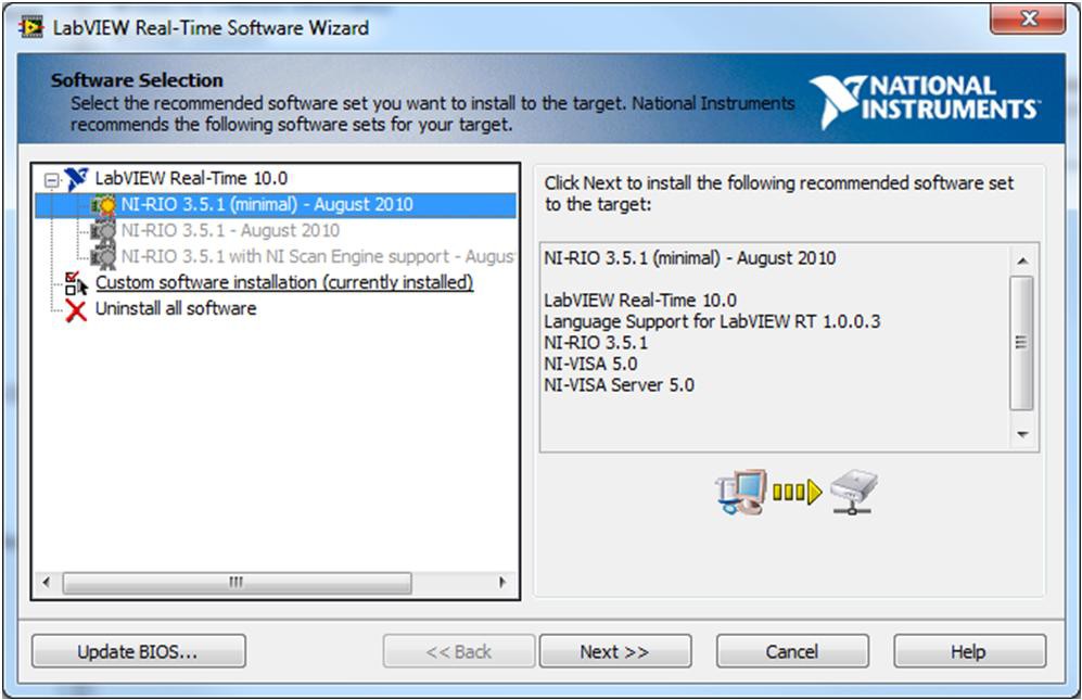
Support for network streams when developing applications for LabVIEW Real-Time targets is automatically included as part of the installation of the LabVIEW Real-Time Module on the development computer. However, the network streams feature isn’t selected for installation by default when installing software to the Real-Time target from Measurement & Automation Explorer. To enable networks steams with LabVIEW Real-Time targets, ensure the check box for the network streams feature is selected during the installation process as shown below.
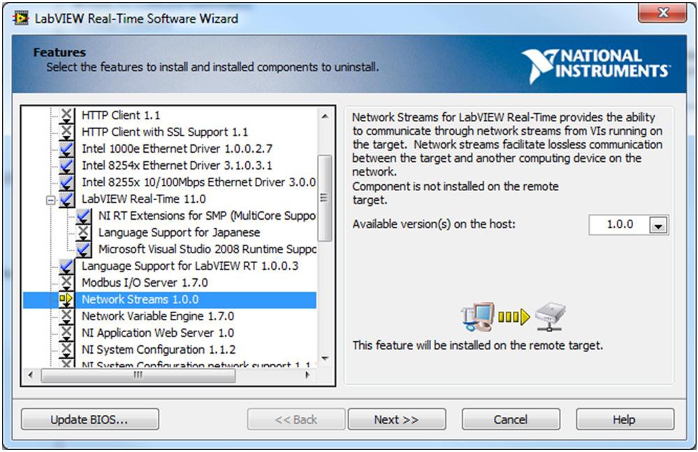
If your Real-Time target provides recommended software sets, network streams may or may not be included as part of the software set. If you don’t see the feature listed as part of the software set, choose another recommended software set that does include the feature or choose the custom software installation option.
Benchmarking Data
In order to provide some guidance on performance expectations, a number of benchmarks were conducted to measure throughput, latency, and CPU utilization of network streams when running on various targets. All benchmarks were conducted on an isolated Gigabit network. If either of the targets involved in the communication doesn’t support a 1 Gb/s network interface, the network connection will automatically negotiate down to 100 Mb/s. A high level summary of the specifications for each of the targets involved in the benchmarks is shown in the table below.
Controller | Processor | Memory | Network Interface | Software |
| Desktop PC | Intel Xeon Quad-Core W3520, 2.66 GHz | 6 GB | 1 Gb/s Ethernet Adapter | Windows 7 (64 bit), LabVIEW 2010 (32 bit) |
| NI PXI-8106 | Intel Core 2 Duo, 2.16 GHz | 1 GB | 1 Gb/s Ethernet Adapter | LabVIEW Real-Time 2010 |
| NI cRIO-9012 | 400 MHz Freescale MPC5200 | 64 MB | 100 Mb/s Ethernet Adapter | LabVIEW Real-Time 2010 |
| NI cRIO-9024 | 800 MHz Freescale MPC8377 | 512 MB | 1 Gb/s Ethernet Adapter | LabVIEW Real-Time 2010 |
Unless otherwise noted, all benchmarks were conducted with at least one of the endpoints running on the Desktop PC target. Also, in order to achieve the best networking performance on the PXI-8106 using LabVIEW RT with SMP, the RT SMP CPU Utilities VIs were used to force all system processes to execute on core 0 and all timed structures to execute on core 1.
Throughput
Throughput benchmarks were conducted by transferring a fixed number of Double data elements across the network with each read and write call to the stream. The read and write functions were placed in a loop and executed as fast as the CPU and network would allow. The throughput was then calculated on the reader by counting the total number of elements read from the stream over a 60-second period of time. These measurements were then repeated by switching the direction of the stream in order to quantify any differences in performance when predominantly reading or writing data from a given target.
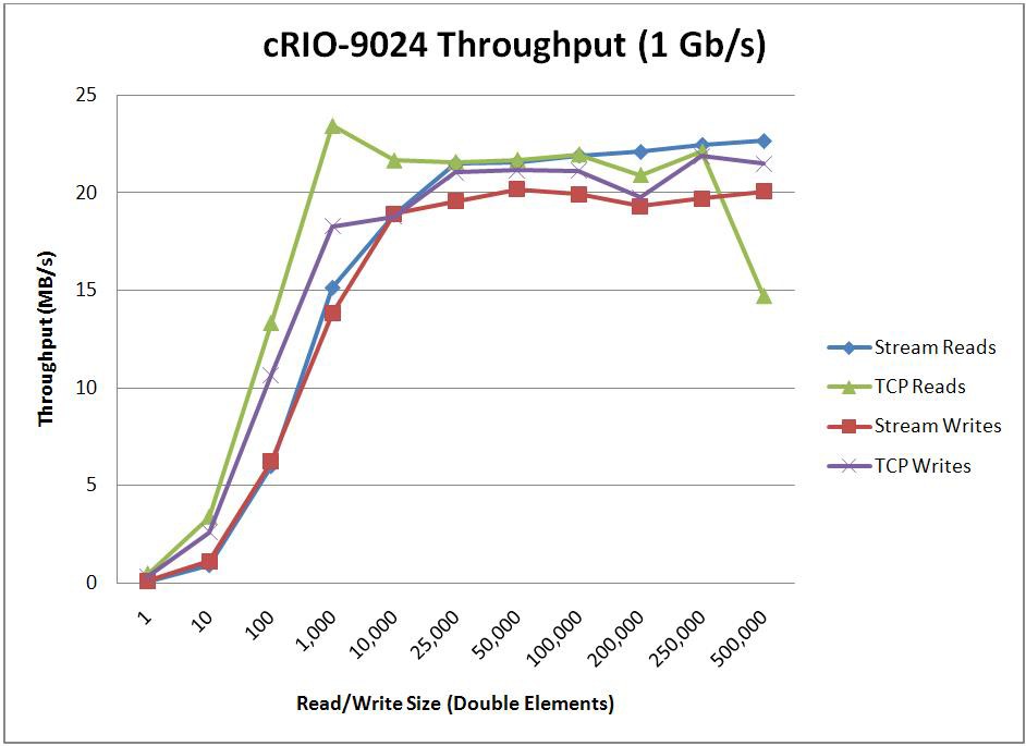
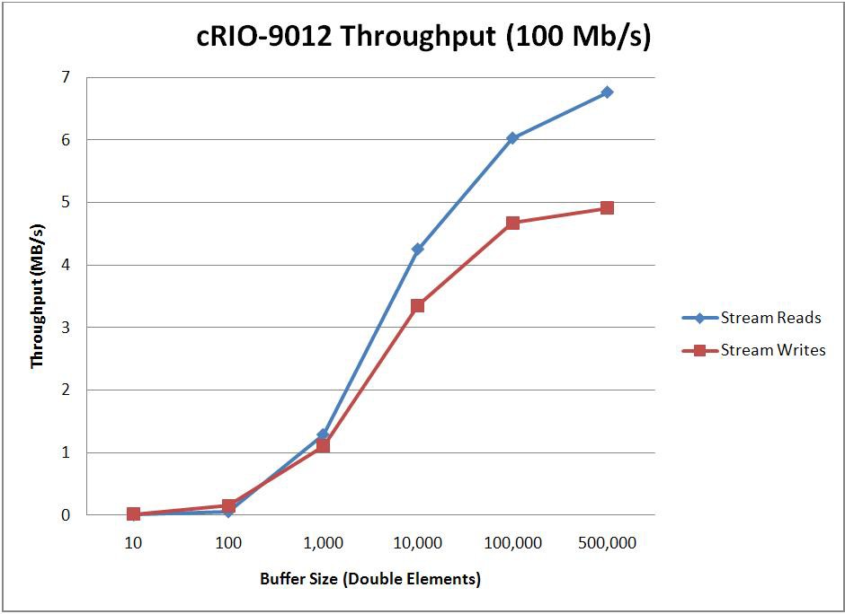
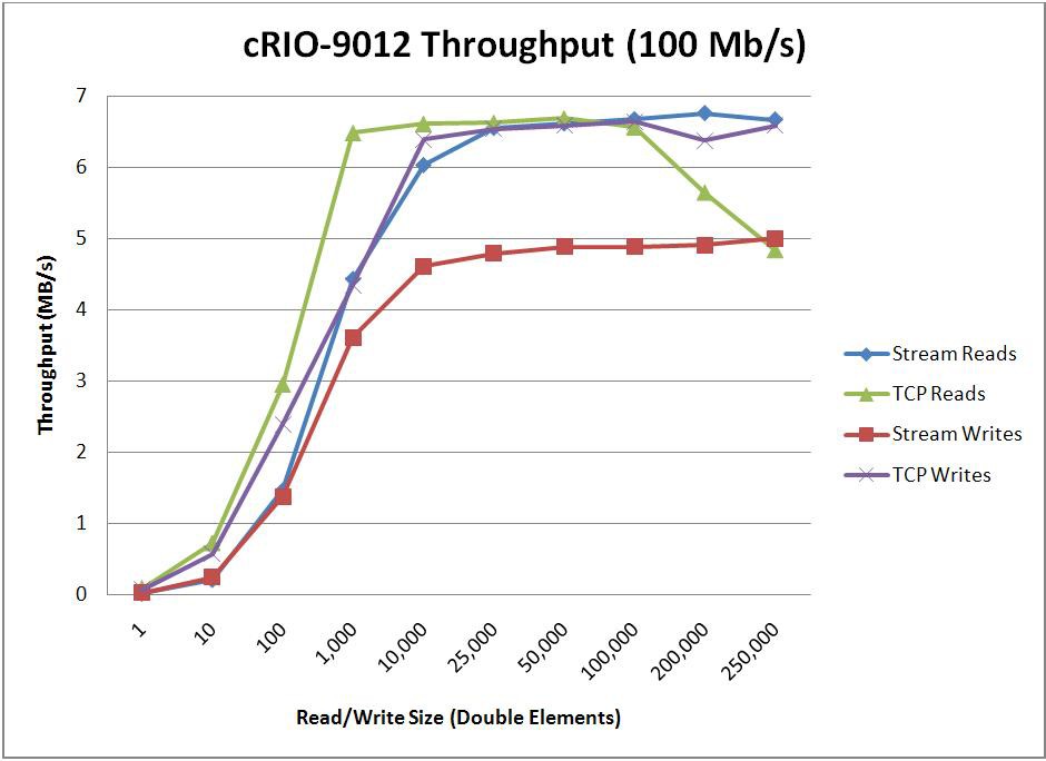
When optimizing for throughput, the endpoint buffer sizes and the number of elements read/written with each read/write call will have a large impact on the throughput that’s achievable. To determine how these parameters impact performance, two tests were conducted. The first test sweeps through various buffer sizes and fixes the read/write size at 1/10th the buffer size. The second test then uses the optimal buffer size found from the first test and sweeps through various read/write sizes. For comparison purposes, this second test was also repeated using TCP functions instead of the Network Streams API. The results of these benchmarks are shown below.
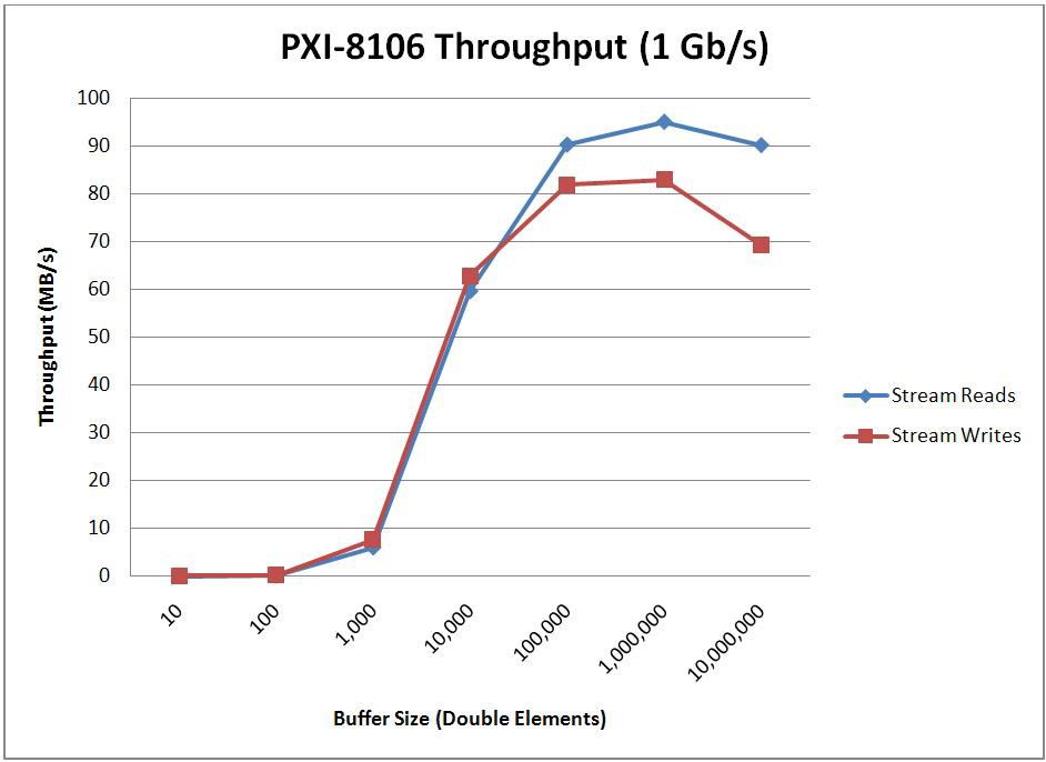

* Stream Endpoint Buffer Size = 1,000,000 Elements
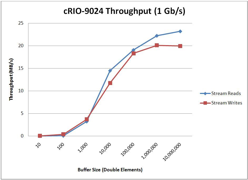
* Stream Endpoint Buffer Size = 1,000,000 Elements
* Stream Endpoint Buffer Size = 500,000 Elements
Latency
Latency benchmarks were conducted by using two streams to form a bidirectional communication link between two targets. The round trip time to write a command from target 1, read the command from target 2, echo the command back to target 1, and read the command back from target 1 was measured. In order to minimize the latency, the flush function was called after each write function. This test sequence was repeated for 10,000 iterations, and the resulting times were then averaged and divided by two to determine the average latency for one-way communication. The measurements were conducted on LabVIEW Real-Time systems to get microsecond resolution and to minimize measurement jitter as much as possible. A similar test was conducted using TCP as the transport mechanism instead of network streams. The results are shown in the table below.
Target | Connection | TCP (µs) | Network Streams (µs) |
| PXI-8106 | 1 Gb/s | 82.02 | 347.90 |
| cRIO-9024 | 1 Gb/s | 268.13 | 630.59 |
| cRIO-9012 | 100 Mb/s | 508.48 | 1581.25 |
Throughput and CPU Usage
To achieve the highest throughput possible, a significant portion of the CPU must often be consumed. In many cases, this is undesirable. Instead, it is often more useful to determine how much throughput can be achieved without exceeding a certain percentage of the overall CPU utilization. In order to obtain this information, a series of benchmarks were conducted to create trend lines between the throughput and the percentage of CPU utilized for each of the various targets. The results of these experiments are shown in the graphs below.
These graphs were produced by writing at a specified rate and measuring the average CPU usage and throughput. For a given throughput rate, the writer would attempt to generate a constant throughput by writing a fixed size amount of data at the time interval required to achieve the desired throughput. Data was then transferred at this target rate for sixty seconds, and CPU utilization was measured every half second throughout the data transfer. At the end of the sixty second interval, the CPU utilization was averaged and the actual throughput was calculated by the reader. The target throughput was then increased, and the process was repeated until either the measured CPU utilization increased above 90 percent or the measured throughput appeared to plateau. The buffer sizes used and the number of elements to read/write per iteration were chosen based on the optimal results from the previous tests. TCP numbers are once again provided as a point of comparison for network streams.
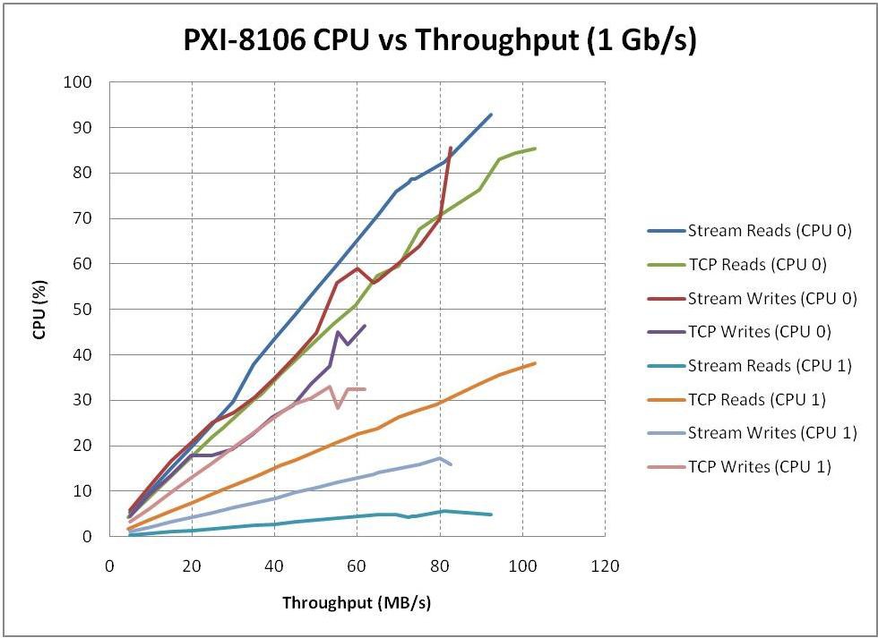
* Stream Buffer Size = 1,000,000 Elements, Stream Read/Write Size = 100,000 Elements, TCP Read/Write Size = 10,000 Elements
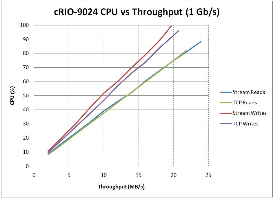
* Stream Buffer Size = 1,000,000 Elements, Stream and TCP Read/Write Size = 100,000 Elements
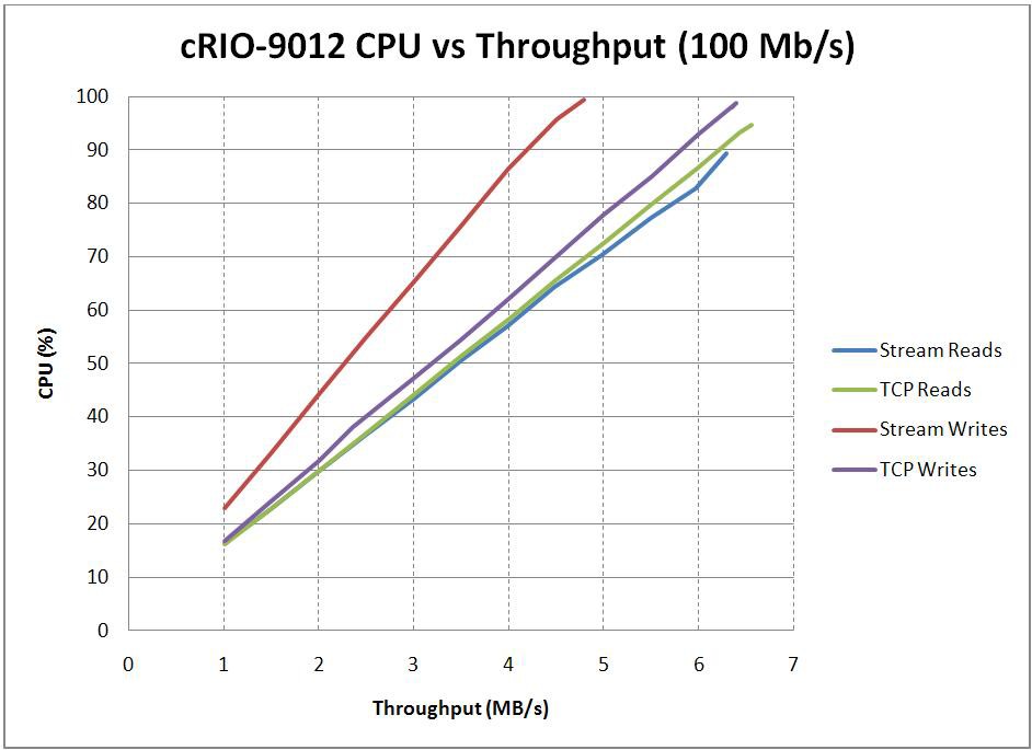
* Stream Buffer Size = 500,000 Elements, Stream and TCP Read/Write Size = 50,000 Elements