RF Simulation Demo: Amplitude Modulation

[ExamplePrograms]

Overview

Modulation is a process by which characteristics of a high-frequency carrier signal are altered to convey information contained in a lower-frequency message. Though it is theoretically possible to transmit baseband signals (or information) without modulating the data, it is far more efficient to send messages by modulating the information onto a carrier wave. High frequency waveforms require smaller antennae for reception, efficiently use available bandwidth, and are flexible enough to carry different types of data. There are a variety of modulation schemes available for both analog and digital modulation.

Background:

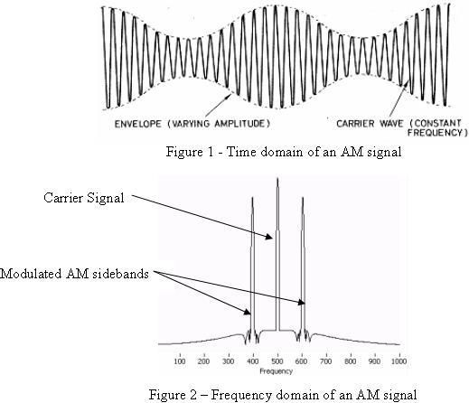
Amplitude Modulation (AM) is an analog modulation scheme where the amplitude (A) of a fixed-frequency carrier signal is continuously modified to represent data in a message.  The carrier signal is generally a high frequency sine wave used to “carry” the information on the envelope of the message.  The result is a double-sideband signal, centered on the carrier frequency, with twice the bandwidth of the original signal.

The following algorithm is commonly used to represent amplitude modulation:

Gathering like terms and simplifying the equation leaves:

y(f) = (C + Msin(ω_mt + φ))sin(ω_ct)

The main advantage of using AM modulation is that it has a very simple circuit implementation (especially for reception), creating widespread adoption quickly.  AM modulation however wastes power and bandwidth in a signal.  The carrier requires the majority of the signal power, but actually does not hold any information.  AM uses twice the required bandwidth by transmitting redundant information in both the upper and lower sidebands.

Programming:

The following steps describe how to build a VI which implements the longer of the two equations shown above for Amplitude Modulation.  Open the “AM Modulation – Medium Exercise.vi”.  Inspect the front panel and block diagram that has already been created for you.  When this VI is completed, you will be able to select the amplitude and frequency of both the carrier and data signals as well as see the time and frequency domain representation of the signals.  The graphs display the behavior of the carrier and sideband signals as modulation parameters (amplitude and frequency) change.  The following front panel represents the operation of a completed VI:

The block diagram consists of a while loop which contains various controls and graphs to display and control the AM signal component information.

1)  Place an “Add” and “Subtract” VI on the block diagram.  Wire the “Carrier Frequency” and “Modulation Frequency” slider controls into the add function.  Wire the  “Carrier Frequency” into the top connector on the subtract function and “Modulation Frequency” into the bottom connector to subtract the two values.

2)  Place a “Simulate Signal” Express VI on the bock diagram.  A dialog box will open to configure the function.  Select the signal type to be a sine wave, set the frequency to 10 Hz, and the amplitude to 1 volt.  Increase the samples per second to be 100000. Deselect the option to automatically select the number of samples, and set the value to also be 100000.  Once you have finished, the dialog box should resemble the image below:

Select the “OK” button.   LabVIEW will now generate all of the code required for this function.  Make three copies of the function by selecting the VI on the block diagram and holding CTRL while dragging the cursor to an open area.  For the first Simulate Signal VI, wire the Carrier Amplitude into amplitude input and Carrier Frequency into frequency input.  For the second Simulate Signal VI, wire the output of the add function into the frequency input. Wire a constant value of 1 into the amplitude input by right-clicking on the connector and selecting “Create>>Constant”.  For the third Simulate Signal VI, wire the output of the subtract function into the frequency input.  Again, wire a constant value of 1 into the amplitude input by right-clicking on the connector and selecting “Create>>Constant”. 

3)  Place a “Multiply” VI on the block diagram.  Wire the sine wave outputs of the second and third Simulate Signal VIs into the multiply function.  Wire the output of the Multiply function into the Modulated Signal graph.  Also, wire the output of the first Simulate Signal VI into the Carrier Signal graph.

4)  Place a “Divide” VI on the block diagram.  Right-click on the lower input connector and create a constant value of 2.  Highlight the constant and the divide function on the block diagram and make a copy by holding CTRL while dragging the cursor to an open area.  Wire the input of one of the divide functions to the output of the second Simulate Signal VI.  Wire the input of the other divide functions to the output of the third Simulate Signal VI.

5)  Place two “Multiply” VIs on the block diagram.  Wire the Modulation Amplitude control and the output of one of the divide functions into the first multiply function.  Wire the output of the second Divide function and the Modulation Amplitude control into the second multiply function.

6)  Place a “Subtract” VI on the block diagram and wire the outputs of both of the multiply functions from the last step into the inputs.  Connect the inputs so the data from the second Simulate Signal VI is being subtracted from the third Simulate Signal VI.

7)  Place an “Add” VI on the block diagram and wire the output of the subtract function from the last step into the function.  Also wire the output from the first Simulate Signal VI into the add function. 

😎  Place a “Spectral Measurements” Express VI on the block diagram.  A dialog box will open to configure the function.  Select the spectral measurement to be magnitude (peak) in dB.  Set the Window to be “7 Term B-Harris” (do not enable averaging).  Once you have finished, the dialog box should resemble the image below:

Select the OK button.  LabVIEW will now generate the code for the function.   Wire the output of the add function from the previous step in the signals input connector.  Also wire the output of the add function to the AM Modulated Signal (Time Domain) graph.  Finally wire the output of the Spectral Measurements Express VI to the AM Modulated Signal (Frequency Domain) graph.

Your VI is now complete.  The block diagram of the completed program should resemble the image below.  Press the run icon to execute your VI.  Vary the values for the carrier and modulation amplitude and frequency to see the effect it has on the signal.